1. Multi-head (Self/Cross) Attention#

本节我们继续介绍 Transformer 架构的多头（自/交叉）注意力。下面是 Multi-head Attention 的架构图：

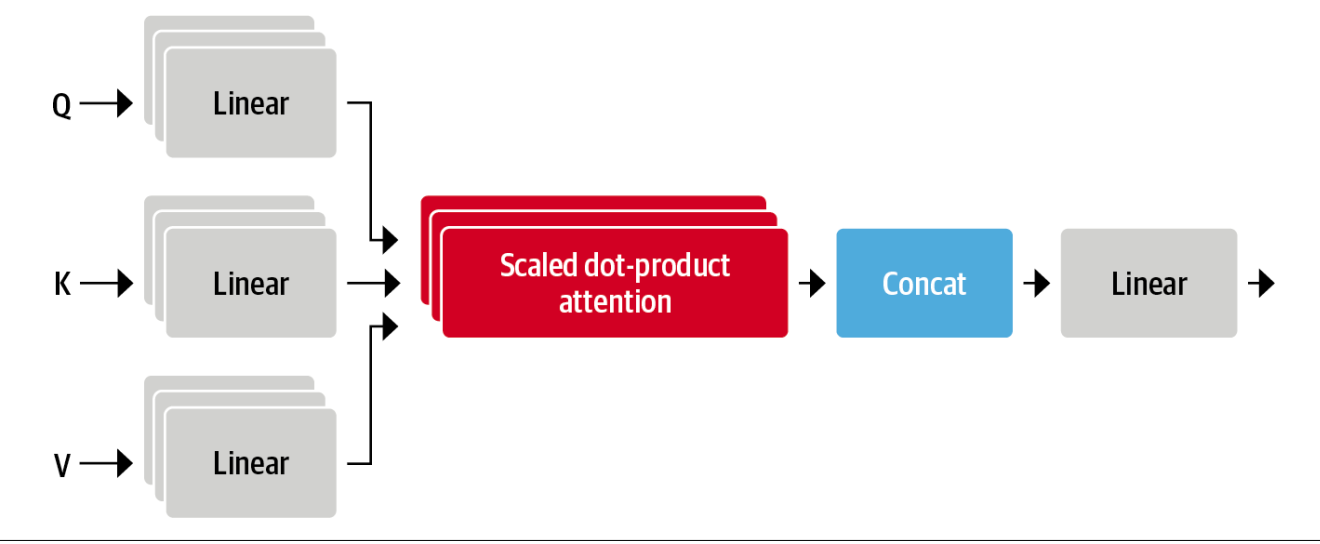
多个头的 Scaled dot product attention 拼接起来，送给 concat，然后交给 Linear 就得到了 multi-head attention 的输出。

我们首先承接上一节的内容：

1
import torch
2
from torch import nn
3
import transformers
4
import numpy as np
5
import pandas as pd
6
import matplotlib.pyplot as plt
7
import matplotlib as mpl
8

9
mpl.rcParams['figure.dpi'] = 200

1
print(torch.__version__) # 2.6.0+cu124
2
print(transformers.__version__) # 5.9.0

1
from transformers import AutoTokenizer

1
from bertviz.transformers_neuron_view import BertModel
2
from bertviz.neuron_view import show

1
model_ckpt = 'bert-base-uncased'
2
tokenizer = AutoTokenizer.from_pretrained(model_ckpt)
3

4
model = BertModel.from_pretrained(model_ckpt)

1
model

1
sample_text = 'time flies like an arrow'
2

3
show(
4
    model,
5
    model_type='bert',
6
    tokenizer=tokenizer,
7
    sentence_a=sample_text,
8
    display_mode='light',
9
    layer=0,
10
    head=8
11
    )

1
model_inputs = tokenizer(sample_text, return_tensors='pt', add_special_tokens=False)
2
model_inputs

1
from torch import nn
2
from transformers import AutoConfig

1
config = AutoConfig.from_pretrained(model_ckpt)
2
config

1
# config.vocab_size: 30522
2
# config.hidden_size: 768=64*12
3
token_embedding = nn.Embedding(config.vocab_size, config.hidden_size)
4
token_embedding # Embedding(30522, 768)

1
# forward of embedding module
2
input_embeddings = token_embedding(model_inputs['input_ids'])
3

4
# batch_size, seq_len, hidden_size
5
input_embeddings.shape # torch.Size([1, 5, 768])

1
# 先不考虑 position encoding
2
# query: [1, 5, 768], key: [1, 5, 768], value: [1, 5, 768]
3
# W_q, W_k, W_v: nn.linear, 作用在 token_embedding 上，依然通过 learing 最终决定
4
query = key = value = input_embeddings
5
dim_k = key.size(-1) # 768
6
print(dim_k)
7

8
# /np.sqrt(dim_k) 是为了缩放，防止 dot product 过大导致 softmax 后梯度消失
9
attention_scores = torch.matmul(query, key.transpose(1, 2)) / np.sqrt(dim_k)
10
attention_scores.shape # torch.Size([1, 5, 5])
11
attention_scores

1
# from scores -> weights, softmax
2
import torch.nn.functional as F
3

4
attention_weights = F.softmax(attention_scores, dim=-1)
5
attention_weights.shape # torch.Size([1, 5, 5])
6
attention_weights

1
attention_weights.sum(dim=-1) # 每行加起来等于 1

1
# 5*5, 5*768 -> 5*768
2
attention_output = torch.bmm(attention_weights, value)
3
attention_output.shape # torch.Size([1, 5, 768])
4
attention_output

1
# batch_size, seq_len, hidden_size
2
def scaled_dot_product_attention(query, key, value):
3
    dim_k = key.size(-1)
4
    attention_scores = torch.matmul(query, key.transpose(1, 2)) / np.sqrt(dim_k)
5
    attention_weights = F.softmax(attention_scores, dim=-1)
6
    attention_output = torch.bmm(attention_weights, value)
7
    return attention_output

1
scaled_dot_product_attention(query, key, value)

以上就是上一节的内容，这里我们已经得到了 Scaled dot product attention，也就是之前示意图中的红色部分。

下面正式进入本节的部分。

1
class AttentionHead(nn.Module):
2
    def __init__(self, embed_dim, head_dim):
3
        super().__init__()
4
        # 三个线性层，用 W 把输入投影成 query, key, value
5
        self.W_q = nn.Linear(embed_dim, head_dim)
6
        self.W_k = nn.Linear(embed_dim, head_dim)
7
        self.W_v = nn.Linear(embed_dim, head_dim)
8

9
    def forward(self, hidden_states):
10
        q = self.W_q(hidden_states)
11
        k = self.W_k(hidden_states)
12
        v = self.W_v(hidden_states)
13
        attention_output = scaled_dot_product_attention(q, k, v)
14
        return attention_output

我们这里简单定义了一个注意力头从输入到输出的完整 pipline. 这里的 W_q, W_k, W_v 是 nn.Linear 模块，每个模块内部存储着：

一个可学习的权重矩阵 weight，形状为 (head_dim, embed_dim)
一个可学习的 bias，形状为 (head_dim)，默认开启

那么我们在上一节中提到的，数学上的 $W^Q$ 对应的就是 self.W_q.weight，再加上可选的 bias.

关于具体得到 $Q,K,V$ 的过程，我们知道 hidden_states 的形状为 [batch_size, seq_len, embed_dim]. 对于每个 token 位置 $i$ ，它的向量为 $x_i$ （长度 768），那么 nn.Linear 对每个 $x_i$ 做的就是：

q_i=W^Qx_i+b^Q

在 Pytorch 中，nn.Linear(in_features, out_features) 的 forward 本质是

y=xW^T+b

其中 $W$ 的形状是 (out_features, in_features)，也就是 (head_dim, embed_dim)，差别主要是 PyTorch 把权重存成 (out, in)，关于这一点我们在 08 节中探讨过。

对整段序列，PyTorch 会在 batch 和 seq_len 维上批量做同样的线性变换，所以一次调用就得到所有位置的 $Q$ :

1
hidden_states: [batch, seq_len, embed_dim]
2
        ↓  W_q（对每个 token 的向量做同一线性变换）
3
q:             [batch, seq_len, head_dim]

$K,V$ 同理。

1
class MultiHeadAttention(nn.Module):
2
    # config 见前文，存储 BERT 的超参数
3
    def __init__(self, config):
4
        super().__init__()
5
        embed_dim = config.hidden_size          # 例如 BERT-base: 768
6
        num_heads = config.num_attention_heads  # 例如 12
7
        head_dim = embed_dim // num_heads       # 768 // 12 = 64
8
        self.heads = nn.ModuleList([
9
            AttentionHead(embed_dim, head_dim) for _ in range(num_heads)
10
        ])
11
        self.output_layer = nn.Linear(embed_dim, embed_dim)
12

13
    # 定义前向计算过程
14
    def forward(self, hidden_states):
15
        # hidden_states: [batch_size, seq_len, embed_dim]
16
        # 按头分割
17
        # 每个头得到的结果是 [batch_size, seq_len, head_dim]
18
        x = torch.cat([head(hidden_states) for head in self.heads], dim=-1)
19
        x = self.output_layer(x)
20
        return x

这里我们就定义了多头注意力，它的核心之前也介绍过：不要只算一次注意力，而是并行算多个独立的注意力头，每个头用自己的 $W^Q, W^K, W^V$ ，从不同子空间看同一段序列；再把各头结果拼起来，最后过一个线性层得到输出。

nn.ModuleList ：把多个子模块放进列表，PyTorch 能正确注册参数。
- 列表里有 12 个 AttentionHead，彼此参数不共享。
- 每个 AttentionHead 内部有 3 个 nn.Linear(embed_dim, head_dim)，即各自的 $W^Q, W^K, W^V$ .
torch.cat ：对得到的 12 个 tensors 进行拼接，dim=-1 表示在 特征维 上拼接：

1
head_0:  [B, L, 64]
2
head_1:  [B, L, 64]
3
...
4
head_11: [B, L, 64]
5
         ↓ concat
6
x:       [B, L, 768]    # 64 × 12 = 768

x = self.output_layer(x) ：最后输出线性层，对每个 token 的 768 维向量做 $y=xW^O+b$ ，最终返回的 x 就是 Multi-head Attention 的输出。

整体的数据流：

1
hidden_states                    [B, L, 768]
2
        │
3
        ├─ AttentionHead 0 ──→ [B, L, 64]
4
        ├─ AttentionHead 1 ──→ [B, L, 64]
5
        ├─ ...
6
        └─ AttentionHead 11 ─→ [B, L, 64]
7
        │
8
        ▼ torch.cat(dim=-1)
9
        x                            [B, L, 768]
10
        │
11
        ▼ output_layer (W^O)
12
        输出                           [B, L, 768]

1
from torch import nn
2
from transformers import AutoConfig, AutoTokenizer, AutoModel
3

4
model_ckpt = 'bert-base-uncased'
5
tokenizer = AutoTokenizer.from_pretrained(model_ckpt)
6

7
# hyperparameters
8
config = AutoConfig.from_pretrained(model_ckpt)
9
config

1
mha = MultiHeadAttention(config)

1
# input
2
# config.vocab_size: 30522
3
# config.hidden_state: 768=64*12
4
# lookup-table, learnable
5
token_embedding = nn.Embedding(config.vocab_size, config.hidden_size)
6
# token_embedding
7
sample_text = 'time flies like an arrow'
8
model_inputs = tokenizer(sample_text, return_tensors='pt', add_special_tokens=False)
9
# foward of embedding module
10
input_embeddings = token_embedding(model_inputs['input_ids'])
11
# batch_size, seq_len, hidden_size
12
input_embeddings.shape # torch.Size([1, 5, 768])

1
mha(input_embeddings)

输出为：

1
tensor([[[ 0.3316, -0.1109, -0.2945,  ...,  0.2417, -0.0272,  0.0901],
2
         [ 0.3491, -0.1779, -0.2362,  ...,  0.1970,  0.1125,  0.0460],
3
         [ 0.2233, -0.0979, -0.1581,  ...,  0.1129,  0.1000,  0.0995],
4
         [ 0.3722, -0.1765, -0.2382,  ...,  0.1719, -0.0061,  0.0895],
5
         [ 0.3137, -0.2047, -0.2799,  ...,  0.2113,  0.0330, -0.0451]]],
6
       grad_fn=<ViewBackward0>)

1
from bertviz import head_view
2
from transformers import AutoModel
3

4
model = AutoModel.from_pretrained(model_ckpt, output_attentions=True)
5
sentence_a = 'time flies like an arrow'
6
sentence_b = 'fruit flies like a banana'
7
viz_inputs = tokenizer(sentence_a, sentence_b, return_tensors='pt')
8

9
# nsp (next sentence prediction)
10
print(viz_inputs)
11
attention = model(**viz_inputs).attentions
12
sentence_b_start = (viz_inputs.token_type_ids == 0).sum(dim=1)
13
print(sentence_b_start)
14

15
tokens = tokenizer.convert_ids_to_tokens(viz_inputs.input_ids[0]) # tensor([...])
16
head_view(attention, tokens, sentence_b_start, heads=[8])

部分输出为：

1
{'input_ids': tensor([[  101,  2051, 10029,  2066,  2019,  8612,   102,  5909, 10029,  2066,
2
          1037, 15212,   102]]), 'token_type_ids': tensor([[0, 0, 0, 0, 0, 0, 0, 1, 1, 1, 1, 1, 1]]), 'attention_mask': tensor([[1, 1, 1, 1, 1, 1, 1, 1, 1, 1, 1, 1, 1]])}
3
tensor([7])

可以看出，我们只有一个 tensor，也就是说两句话实际上被展平了，我们识别第一句话和第二句话的方法就是看 token_type_ids，为 0 的就是第一句话，为 1 的就是第二句话。

音乐

音乐

1. Multi-head (Self/Cross) Attention#

文章分享

评论区

音乐

文章目录

音乐

音乐

03_transformer_architecture_multi_head_attention

1. Multi-head (Self/Cross) Attention#

文章分享

评论区

音乐

文章目录