1
from transformers import BertModel, BertForSequenceClassification

1
model_name = 'bert-base-uncased'
2
model = BertModel.from_pretrained(model_name)
3
cls_model = BertForSequenceClassification.from_pretrained(model_name)

1
model

输出为：

1
BertModel(
2
  (embeddings): BertEmbeddings(
3
    (word_embeddings): Embedding(30522, 768, padding_idx=0)
4
    (position_embeddings): Embedding(512, 768)
5
    (token_type_embeddings): Embedding(2, 768)
6
    (LayerNorm): LayerNorm((768,), eps=1e-12, elementwise_affine=True, bias=True)
7
    (dropout): Dropout(p=0.1, inplace=False)
8
  )
9
  (encoder): BertEncoder(
10
    (layer): ModuleList(
11
      (0-11): 12 x BertLayer(
12
        (attention): BertAttention(
13
          (self): BertSelfAttention(
14
            (query): Linear(in_features=768, out_features=768, bias=True)
15
            (key): Linear(in_features=768, out_features=768, bias=True)
16
            (value): Linear(in_features=768, out_features=768, bias=True)
17
            (dropout): Dropout(p=0.1, inplace=False)
18
          )
19
          (output): BertSelfOutput(
20
            (dense): Linear(in_features=768, out_features=768, bias=True)
21
            (LayerNorm): LayerNorm((768,), eps=1e-12, elementwise_affine=True, bias=True)
22
            (dropout): Dropout(p=0.1, inplace=False)
23
          )
24
        )
25
        (intermediate): BertIntermediate(
26
          (dense): Linear(in_features=768, out_features=3072, bias=True)
27
          (intermediate_act_fn): GELUActivation()
28
        )
29
        (output): BertOutput(
30
          (dense): Linear(in_features=3072, out_features=768, bias=True)
31
          (LayerNorm): LayerNorm((768,), eps=1e-12, elementwise_affine=True, bias=True)
32
          (dropout): Dropout(p=0.1, inplace=False)
33
        )
34
      )
35
    )
36
  )
37
  (pooler): BertPooler(
38
    (dense): Linear(in_features=768, out_features=768, bias=True)
39
    (activation): Tanh()
40
  )
41
)

1.1 `BertModel` 的架构#

当你在 HuggingFace Transformers 中打印一个 BertModel 对象时，它会递归显示模型的所有模块层（modules/layers），就像一个层层嵌套的目录树。每个缩进代表一层封装，每个 () 里的内容就是一个 PyTorch 的 nn.Module 子模块。

简单来说，这就是在展示 BERT 模型的「骨架图」—— 从最外层到最内层的每一个神经网络层。

BERT-base 由 3 大块组成：

Embeddings（嵌入层）—— 把文本转成向量：把输入的 token ID 转换成 768 维的稠密向量，并加上位置信息。

1
(embeddings): BertEmbeddings(
2
  (word_embeddings): Embedding(30522, 768)       # 词表大小 30522 → 768 维向量
3
  (position_embeddings): Embedding(512, 768)      # 位置编码，最多 512 个位置
4
  (token_type_embeddings): Embedding(2, 768)      # 句子类型（两句任务用）
5
  (LayerNorm): LayerNorm(768)                      # 层归一化
6
  (dropout): Dropout(p=0.1)                        # 随机丢弃 10% 防止过拟合
7
)

Encoder（编码器）—— 核心 Transformer 层

1
(encoder): BertEncoder(
2
  (layer): ModuleList(
3
    (0-11): 12 x BertLayer( ... )    # 12 层完全相同的 Transformer 块
4
  )
5
)

每层 BertLayer 又由 3 个子模块组成：

Attention（注意力机制）：让每个词「看到」句子中所有其他词，学习上下文关系。

1
(attention): BertAttention(
2
  (self): BertSelfAttention(          # 多头自注意力
3
    (query/key/value): Linear(768→768)  # Q、K、V 三个线性变换
4
    (dropout): Dropout(p=0.1)
5
  )
6
  (output): BertSelfOutput(            # 注意力输出
7
    (dense): Linear(768→768)
8
    (LayerNorm): LayerNorm(768)
9
    (dropout): Dropout(p=0.1)
10
  )
11
)

Intermediate（中间层）

1
(intermediate): BertIntermediate(
2
  (dense): Linear(768 → 3072)         # 扩展到 4 倍维度
3
  (intermediate_act_fn): GELUActivation()  # GELU 激活函数
4
)

Output（输出层）

1
(output): BertOutput(
2
  (dense): Linear(3072 → 768)         # 压缩回 768 维
3
  (LayerNorm): LayerNorm(768)
4
  (dropout): Dropout(p=0.1)
5
)

中间层和输出层合称 FFN（前馈神经网络）：先扩张再压缩，增加模型的表达能力。

Pooler（汇聚层）—— 提取 [CLS] 向量：取出编码器输出中第一个位置 [CLS] 的向量，再经过一层线性变换 + tanh，作为整句话的语义表示，常用于分类任务。

1
(pooler): BertPooler(
2
  (dense): Linear(768 → 768)
3
  (activation): Tanh()                # tanh 激活
4
)

整体架构示意图：

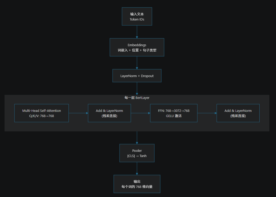
这个架构就是 BERT 的核心：双向的 Transformer 编码器，通过 MLM（遮蔽语言模型）和 NSP（下一句预测）两个任务进行预训练，学到了丰富的语言知识。

1
cls_model

输出为：

1
BertForSequenceClassification(
2
  (bert): BertModel(
3
    (embeddings): BertEmbeddings(
4
      (word_embeddings): Embedding(30522, 768, padding_idx=0)
5
      (position_embeddings): Embedding(512, 768)
6
      (token_type_embeddings): Embedding(2, 768)
7
      (LayerNorm): LayerNorm((768,), eps=1e-12, elementwise_affine=True, bias=True)
8
      (dropout): Dropout(p=0.1, inplace=False)
9
    )
10
    (encoder): BertEncoder(
11
      (layer): ModuleList(
12
        (0-11): 12 x BertLayer(
13
          (attention): BertAttention(
14
            (self): BertSelfAttention(
15
              (query): Linear(in_features=768, out_features=768, bias=True)
16
              (key): Linear(in_features=768, out_features=768, bias=True)
17
              (value): Linear(in_features=768, out_features=768, bias=True)
18
              (dropout): Dropout(p=0.1, inplace=False)
19
            )
20
            (output): BertSelfOutput(
21
              (dense): Linear(in_features=768, out_features=768, bias=True)
22
              (LayerNorm): LayerNorm((768,), eps=1e-12, elementwise_affine=True, bias=True)
23
              (dropout): Dropout(p=0.1, inplace=False)
24
            )
25
          )
26
          (intermediate): BertIntermediate(
27
            (dense): Linear(in_features=768, out_features=3072, bias=True)
28
            (intermediate_act_fn): GELUActivation()
29
          )
30
          (output): BertOutput(
31
            (dense): Linear(in_features=3072, out_features=768, bias=True)
32
            (LayerNorm): LayerNorm((768,), eps=1e-12, elementwise_affine=True, bias=True)
33
            (dropout): Dropout(p=0.1, inplace=False)
34
          )
35
        )
36
      )
37
    )
38
    (pooler): BertPooler(
39
      (dense): Linear(in_features=768, out_features=768, bias=True)
40
      (activation): Tanh()
41
    )
42
  )
43
  (dropout): Dropout(p=0.1, inplace=False)
44
  (classifier): Linear(in_features=768, out_features=2, bias=True)
45
)

1.2 BertForSequenceClassification 的输出#

BertModel（基础模型）的架构：

1
BertModel
2
├── embeddings
3
├── encoder (12× BertLayer)
4
└── pooler

BertForSequenceClassification（分类模型）的架构：

1
BertForSequenceClassification
2
├── bert (整个 BertModel)
3
│   ├── embeddings
4
│   ├── encoder (12× BertLayer)
5
│   └── pooler
6
├── dropout
7
└── classifier: Linear(768 → 2)

对比如下：

对比项	`BertModel`	`BertForSequenceClassification`
结构	只有 backbone	在 backbone 基础上 + 分类头
额外模块	无	`dropout` + `classifier: Linear(768 → 2)`
输出	所有 token 的 768 维向量 + pooler 输出	2 个类别的 logits（如正面/负面）
用途	通用特征提取器	专用于文本分类任务

新增的两个模块：

dropout —— 随机丢弃 10% 的神经元，防止微调时过拟合。
classifier: Linear(768 → 2) —— 将 pooler 输出的 [CLS] 向量（768 维）映射到 2 个分类标签上。

为什么这样设计？

这背后是 “预训练 + 微调”（Pre-train then Fine-tune）范式：

1
预训练阶段:       BertModel (在大规模无标注语料上学习通用语言知识)
2
                       ↓
3
微调阶段:    BertForSequenceClassification (用标注数据微调整个模型)

BertModel 就像是一个通用的「语言理解引擎」，通过 MLM 和 NSP 任务学会了词法、句法和语义知识，但它本身不针对任何具体任务。
BertForSequenceClassification 则是在这个引擎上加了一个「任务专用头」（classifier head），用于具体的分类任务（如情感分析、垃圾邮件检测等）。
微调时，整个模型（bert backbone + 分类头）一起训练。Bert 部分做微小的参数调整来适配任务，而新加的 classifier 层则从头学习如何将 [CLS] 语义向量映射到目标类别。
in_features=768 的 768 正是 BertModel 的 hidden_size，而 out_features=2 表示该任务有 2 个分类（例如正面/负面）。

简单类比：BertModel 像是一个大学毕业生（通才），BertForSequenceClassification 像是在这个毕业生基础上进行「岗前培训」，让他成为某个特定岗位的专家（专才）。

1.3 为什么 BERT 没有 decoder#

先回顾一下原始 Transformer 和 BERT 的关系：

1.3.1 原始 Transformer = Encoder + Decoder#

原始的 Transformer（2017 年由 Google 提出）是 Encoder-Decoder 架构，专门用于序列到序列（seq2seq）任务，比如机器翻译：

1
原始 Transformer
2
├── Encoder（编码器：6层） ← 双向注意力（能看到所有词）
3
└── Decoder（解码器：6层） ← 掩码注意力（只能看左边的词）

1.3.2 BERT 为什么只用 Encoder？#

因为 BERT 的定位是「语言理解」模型，而不是「语言生成」模型。具体来说：

1. 预训练任务决定了架构#

模型	预训练任务	需要什么能力	选用哪部分
BERT	MLM（遮蔽语言模型）+ NSP	理解上下文 → 预测被遮住的词	Encoder（双向上下文）
GPT	自回归语言模型（预测下一个词）	从左到右依次生成	Decoder（单向因果注意力）
T5 / BART	去噪自编码（如翻译、文本修复）	理解输入 + 生成输出	Encoder + Decoder

MLM 任务：随机遮住 15% 的词，让模型根据左右两边的上下文来预测被遮住的词。
这就要求模型能同时看到某个词的左边和右边的信息——这正是 Encoder 的双向自注意力（bidirectional self-attention）的特性。

2. Decoder 的因果掩码（Causal Mask）不适合 BERT#

Decoder 的核心特点是 因果注意力（causal attention）：每个 token 只能看到它自己和它左边的 token，看不到右边的 token。这是为了在生成时保证自回归性质（不能偷看未来的词）。

但 BERT 的任务（MLM）恰恰需要看到未来的词（右边的上下文）来预测当前遮住的词，所以 Decoder 的因果掩码反而会阻碍 BERT 的学习目标。

一张图总结：不同模型家族的架构选择

graph LR subgraph "原始 Transformer" E[Encoder 双向注意力] D[Decoder 因果注意力] end subgraph "理解派 (Encoder-only)" B[BERT RoBERTa ALBERT] end subgraph "生成派 (Decoder-only)" G[GPT LLaMA Qwen] end subgraph "翻译/转换派 (Encoder-Decoder)" T[T5 BART mT5] end E --> B D --> G E --> T D --> T

流派	代表模型	使用部分	典型任务
Encoder-only	BERT, RoBERTa, ALBERT	只用 Encoder	文本分类、情感分析、NER、阅读理解
Decoder-only	GPT, LLaMA, Qwen	只用 Decoder	文本生成、对话、代码生成
Encoder-Decoder	T5, BART, mT5	Encoder + Decoder	翻译、摘要、文本修复

1.3.3 一句话总结#

BERT 只用 Encoder 是因为它的目标是「理解」而不是「生成」——需要同时看左右上下文来理解语义，而这正是 Encoder 双向注意力的专长。Decoder 的因果掩码（只能看左边）反而会限制这种理解能力。

2. 参数统计#

total_params ：总参数量
total__learnable_params ：可学习参数量

2.1 参数形状#

1
for name, param in model.named_parameters():
2
    print(name, '->', param.shape)

输出为：

1
embeddings.word_embeddings.weight -> torch.Size([30522, 768])
2
embeddings.position_embeddings.weight -> torch.Size([512, 768])
3
embeddings.token_type_embeddings.weight -> torch.Size([2, 768])
4
embeddings.LayerNorm.weight -> torch.Size([768])
5
embeddings.LayerNorm.bias -> torch.Size([768])
6
encoder.layer.0.attention.self.query.weight -> torch.Size([768, 768])
7
encoder.layer.0.attention.self.query.bias -> torch.Size([768])
8
encoder.layer.0.attention.self.key.weight -> torch.Size([768, 768])
9
encoder.layer.0.attention.self.key.bias -> torch.Size([768])
10
encoder.layer.0.attention.self.value.weight -> torch.Size([768, 768])
11
encoder.layer.0.attention.self.value.bias -> torch.Size([768])
12
encoder.layer.0.attention.output.dense.weight -> torch.Size([768, 768])
13
encoder.layer.0.attention.output.dense.bias -> torch.Size([768])
14
encoder.layer.0.attention.output.LayerNorm.weight -> torch.Size([768])
15
encoder.layer.0.attention.output.LayerNorm.bias -> torch.Size([768])
16
encoder.layer.0.intermediate.dense.weight -> torch.Size([3072, 768])
17
encoder.layer.0.intermediate.dense.bias -> torch.Size([3072])
18
encoder.layer.0.output.dense.weight -> torch.Size([768, 3072])
19
encoder.layer.0.output.dense.bias -> torch.Size([768])
20
encoder.layer.0.output.LayerNorm.weight -> torch.Size([768])
21
encoder.layer.0.output.LayerNorm.bias -> torch.Size([768])
22
encoder.layer.1.attention.self.query.weight -> torch.Size([768, 768])
23
encoder.layer.1.attention.self.query.bias -> torch.Size([768])
24
encoder.layer.1.attention.self.key.weight -> torch.Size([768, 768])
25
encoder.layer.1.attention.self.key.bias -> torch.Size([768])
26
...
27
encoder.layer.11.output.LayerNorm.weight -> torch.Size([768])
28
encoder.layer.11.output.LayerNorm.bias -> torch.Size([768])
29
pooler.dense.weight -> torch.Size([768, 768])
30
pooler.dense.bias -> torch.Size([768])

输出解析：

Embeddings 层（3 个嵌入矩阵 + LayerNorm）
- 前缀 embeddings 说明在哪一层，后面的 word_embeddings 说明在层里的哪个模块中，weight 表示具体的参数是什么。

1
embeddings.word_embeddings.weight       -> [30522, 768]   # 词嵌入矩阵：30522个词 × 768维
2
embeddings.position_embeddings.weight   -> [512, 768]     # 位置嵌入：512个位置 × 768维
3
embeddings.token_type_embeddings.weight -> [2, 768]       # 句子类型嵌入：2种类型 × 768维
4
embeddings.LayerNorm.weight             -> [768]          # LayerNorm 的缩放参数（γ）
5
embeddings.LayerNorm.bias               -> [768]          # LayerNorm 的偏移参数（β）

第 0 层 Encoder 的 Attention 部分（以 layer.0 为例）

1
# Q、K、V 三个线性变换：每个都是 768 → 768
2
encoder.layer.0.attention.self.query.weight   -> [768, 768]   # 权重矩阵 W_q
3
encoder.layer.0.attention.self.query.bias     -> [768]        # 偏置 b_q
4
encoder.layer.0.attention.self.key.weight     -> [768, 768]   # 权重矩阵 W_k
5
encoder.layer.0.attention.self.key.bias       -> [768]        # 偏置 b_k
6
encoder.layer.0.attention.self.value.weight   -> [768, 768]   # 权重矩阵 W_v
7
encoder.layer.0.attention.self.value.bias     -> [768]        # 偏置 b_v
8

9
# 注意力输出层
10
encoder.layer.0.attention.output.dense.weight      -> [768, 768]   # 线性变换
11
encoder.layer.0.attention.output.dense.bias        -> [768]
12
encoder.layer.0.attention.output.LayerNorm.weight  -> [768]
13
encoder.layer.0.attention.output.LayerNorm.bias    -> [768]

第 0 层 Encoder 的 FFN 部分

1
# Intermediate：扩展层 768 → 3072（4倍）
2
encoder.layer.0.intermediate.dense.weight -> [3072, 768]
3
encoder.layer.0.intermediate.dense.bias   -> [3072]
4

5
# Output：压缩层 3072 → 768
6
encoder.layer.0.output.dense.weight       -> [768, 3072]
7
encoder.layer.0.output.dense.bias         -> [768]
8
encoder.layer.0.output.LayerNorm.weight   -> [768]
9
encoder.layer.0.output.LayerNorm.bias     -> [768]

第 1~11 层（结构与 layer.0 完全相同）

1
encoder.layer.1.attention.self.query.weight -> [768, 768]
2
encoder.layer.1.attention.self.key.weight   -> [768, 768]
3
...  # 每一层都重复同样的结构，共 12 层
4
encoder.layer.11.output.LayerNorm.weight    -> [768]
5
encoder.layer.11.output.LayerNorm.bias      -> [768]

Pooler 层

1
pooler.dense.weight -> [768, 768]   # 将 [CLS] 向量再做一次线性变换
2
pooler.dense.bias   -> [768]

核心观察：

观察点	说明	原因
词嵌入矩阵最大	`[30522, 768]` ≈ 2340 万参数	30522 是整个词表大小，这是模型中最大的单一张量
每层结构完全相同	layer.0 ~ layer.11 的参数形状一样	12 层 Transformer 共享同一结构，参数独立
Q/K/V 形状相同	都是 `[768, 768]`	多头注意力中 Q/K/V 维度一致
Intermediate 是 4 倍	`[3072, 768]` = 768 × 4	这是 BERT 的设计惯例：FFN 中间层扩展到 4 倍隐藏维度
线性层的 weight 形状是 `[out, in]`	例如 `[3072, 768]` 表示输出 3072、输入 768	PyTorch 的 `Linear` 层使用 `weight.shape = [out_features, in_features]`

你可以用这个输出手算 BERT-base 的总参数量（约 1.1 亿）：把每个 shape 的元素个数相乘再求和即可。比如 [30522, 768] 就是 30522 × 768 个参数。

2.2 参数量#

1
total_params = 0
2
total_learnable_params = 0
3

4
for name, param in model.named_parameters():
5
    print(name, '->', param.shape, '->', param.numel())
6
    if param.requires_grad:
7
        total_learnable_params += param.numel()
8
    total_params += param.numel()
9

10
print('Total parameters:', total_params)
11
print('Total learnable parameters:', total_learnable_params)

输出为：

1
embeddings.word_embeddings.weight -> torch.Size([30522, 768]) -> 23440896
2
embeddings.position_embeddings.weight -> torch.Size([512, 768]) -> 393216
3
embeddings.token_type_embeddings.weight -> torch.Size([2, 768]) -> 1536
4
embeddings.LayerNorm.weight -> torch.Size([768]) -> 768
5
embeddings.LayerNorm.bias -> torch.Size([768]) -> 768
6
encoder.layer.0.attention.self.query.weight -> torch.Size([768, 768]) -> 589824
7
encoder.layer.0.attention.self.query.bias -> torch.Size([768]) -> 768
8
encoder.layer.0.attention.self.key.weight -> torch.Size([768, 768]) -> 589824
9
encoder.layer.0.attention.self.key.bias -> torch.Size([768]) -> 768
10
encoder.layer.0.attention.self.value.weight -> torch.Size([768, 768]) -> 589824
11
encoder.layer.0.attention.self.value.bias -> torch.Size([768]) -> 768
12
encoder.layer.0.attention.output.dense.weight -> torch.Size([768, 768]) -> 589824
13
encoder.layer.0.attention.output.dense.bias -> torch.Size([768]) -> 768
14
encoder.layer.0.attention.output.LayerNorm.weight -> torch.Size([768]) -> 768
15
encoder.layer.0.attention.output.LayerNorm.bias -> torch.Size([768]) -> 768
16
encoder.layer.0.intermediate.dense.weight -> torch.Size([3072, 768]) -> 2359296
17
encoder.layer.0.intermediate.dense.bias -> torch.Size([3072]) -> 3072
18
encoder.layer.0.output.dense.weight -> torch.Size([768, 3072]) -> 2359296
19
encoder.layer.0.output.dense.bias -> torch.Size([768]) -> 768
20
encoder.layer.0.output.LayerNorm.weight -> torch.Size([768]) -> 768
21
encoder.layer.0.output.LayerNorm.bias -> torch.Size([768]) -> 768
22
encoder.layer.1.attention.self.query.weight -> torch.Size([768, 768]) -> 589824
23
encoder.layer.1.attention.self.query.bias -> torch.Size([768]) -> 768
24
encoder.layer.1.attention.self.key.weight -> torch.Size([768, 768]) -> 589824
25
encoder.layer.1.attention.self.key.bias -> torch.Size([768]) -> 768
26
...
27
pooler.dense.weight -> torch.Size([768, 768]) -> 589824
28
pooler.dense.bias -> torch.Size([768]) -> 768
29
Total parameters: 109482240
30
Total learnable parameters: 109482240

可见，可学习的参数量与总参数量是一致的，接近 1.1 亿。

我们接下来看看每层每个模块的参数量：

1
total_embedding_params = 0
2
total_encoder_params = 0
3
total_pooler_params = 0
4

5
for name, param in model.named_parameters():
6
    if name.startswith('embeddings'):
7
        total_embedding_params += param.numel()
8
    elif name.startswith('encoder'):
9
        total_encoder_params += param.numel()
10
    elif name.startswith('pooler'):
11
        total_pooler_params += param.numel()
12

13
print('Total embedding parameters:', total_embedding_params)
14
print('Total encoder parameters:', total_encoder_params)
15
print('Total pooler parameters:', total_pooler_params)

输出为：

1
Total embedding parameters: 23837184
2
Total encoder parameters: 85054464
3
Total pooler parameters: 590592

下面是占比：

1
params = [total_embedding_params, total_encoder_params, total_pooler_params]
2
for param in params:
3
    print(f'{param / total_params:.2%}')

输出为：

1
21.77%
2
77.69%
3
0.54%

音乐

音乐

1.1 `BertModel` 的架构#

1.2 BertForSequenceClassification 的输出#

1.3 为什么 BERT 没有 decoder#

1.3.1 原始 Transformer = Encoder + Decoder#

1.3.2 BERT 为什么只用 Encoder？#

1. 预训练任务决定了架构#

2. Decoder 的因果掩码（Causal Mask）不适合 BERT#

1.3.3 一句话总结#

2. 参数统计#

2.1 参数形状#

2.2 参数量#

文章分享

评论区

音乐

文章目录

音乐

音乐

03_bert_model_architecture_params

1.1 BertModel 的架构#

1.2 BertForSequenceClassification 的输出#

1.3 为什么 BERT 没有 decoder#

1.3.1 原始 Transformer = Encoder + Decoder#

1.3.2 BERT 为什么只用 Encoder？#

1. 预训练任务决定了架构#

2. Decoder 的因果掩码（Causal Mask）不适合 BERT#

1.3.3 一句话总结#

2. 参数统计#

2.1 参数形状#

2.2 参数量#

文章分享

评论区

音乐

文章目录

1.1 `BertModel` 的架构#