1
from transformers import BertTokenizer, BertModel
2
import torch

1. load model and tokenize#

1
model_type = 'bert-base-uncased'

1
bert = BertModel.from_pretrained(model_type)
2
tokenizer = BertTokenizer.from_pretrained(model_type)

1
text = 'This is a text sentence.'

1
inputs = tokenizer(text, return_tensors='pt')
2
inputs

输出为：

1
{'input_ids': tensor([[ 101, 2023, 2003, 1037, 3793, 6251, 1012,  102]]), 'token_type_ids': tensor([[0, 0, 0, 0, 0, 0, 0, 0]]), 'attention_mask': tensor([[1, 1, 1, 1, 1, 1, 1, 1]])}

1
tokenizer.convert_ids_to_tokens(inputs['input_ids'][0])

输出为：

1
['[CLS]', 'this', 'is', 'a', 'text', 'sentence', '.', '[SEP]']

2. forward and pooler output#

1
bert.eval()

输出为：

1
BertModel(
2
  (embeddings): BertEmbeddings(
3
    (word_embeddings): Embedding(30522, 768, padding_idx=0)
4
    (position_embeddings): Embedding(512, 768)
5
    (token_type_embeddings): Embedding(2, 768)
6
    (LayerNorm): LayerNorm((768,), eps=1e-12, elementwise_affine=True, bias=True)
7
    (dropout): Dropout(p=0.1, inplace=False)
8
  )
9
  (encoder): BertEncoder(
10
    (layer): ModuleList(
11
      (0-11): 12 x BertLayer(
12
        (attention): BertAttention(
13
          (self): BertSelfAttention(
14
            (query): Linear(in_features=768, out_features=768, bias=True)
15
            (key): Linear(in_features=768, out_features=768, bias=True)
16
            (value): Linear(in_features=768, out_features=768, bias=True)
17
            (dropout): Dropout(p=0.1, inplace=False)
18
          )
19
          (output): BertSelfOutput(
20
            (dense): Linear(in_features=768, out_features=768, bias=True)
21
            (LayerNorm): LayerNorm((768,), eps=1e-12, elementwise_affine=True, bias=True)
22
            (dropout): Dropout(p=0.1, inplace=False)
23
          )
24
        )
25
        (intermediate): BertIntermediate(
26
          (dense): Linear(in_features=768, out_features=3072, bias=True)
27
          (intermediate_act_fn): GELUActivation()
28
        )
29
        (output): BertOutput(
30
          (dense): Linear(in_features=3072, out_features=768, bias=True)
31
          (LayerNorm): LayerNorm((768,), eps=1e-12, elementwise_affine=True, bias=True)
32
          (dropout): Dropout(p=0.1, inplace=False)
33
        )
34
      )
35
    )
36
  )
37
  (pooler): BertPooler(
38
    (dense): Linear(in_features=768, out_features=768, bias=True)
39
    (activation): Tanh()
40
  )
41
)

1
with torch.no_grad():
2
    outputs = bert(**inputs)

1
outputs.keys()

输出为：

1
odict_keys(['last_hidden_state', 'pooler_output'])

因为我们没有像在 10 节中那样，往 bert = BertModel.from_pretrained(model_type) 里面传入 output_hidden_states=True 的参数，所以这里只返回两个 keys，没有 hidden_states（参见 10 节）。

1
outputs['last_hidden_state'].shape # torch.Size([1, 8, 768])
2

3
outputs['pooler_output'].shape # torch.Size([1, 768])
4

5
outputs['pooler_output']

输出为：

1
tensor([[-0.9320, -0.4660, -0.7054,  0.8013,  0.5395, -0.2326,  0.8985,  0.3100,
2
         -0.5941, -1.0000, -0.1055,  0.8209,  0.9858,  0.2604,  0.9526, -0.6847,
3
         -0.2648, -0.6366,  0.3471, -0.7114,  0.6518,  0.9998,  0.4752,  0.3604,
4
          0.5276,  0.9401, -0.6821,  0.9463,  0.9627,  0.7596, -0.7972,  0.2211,
5
         -0.9909, -0.2564, -0.7488, -0.9928,  0.4347, -0.8085, -0.0717, -0.0137,
6
         -0.9286,  0.3592,  1.0000, -0.4739,  0.2884, -0.4205, -1.0000,  0.3234,
7
         -0.9190,  0.7232,  0.6715,  0.5167,  0.2301,  0.5236,  0.5461, -0.0622,
8
         -0.0630,  0.1883, -0.2802, -0.6607, -0.6670,  0.3900, -0.6133, -0.9413,
9
          0.5821,  0.5472, -0.1604, -0.3769, -0.1576, -0.0250,  0.9041,  0.2955,
10
         -0.0418, -0.8321,  0.3900,  0.3109, -0.6546,  1.0000, -0.5625, -0.9819,
11
          0.6171,  0.5162,  0.6011,  0.0482,  0.2289, -1.0000,  0.5958, -0.2103,
12
         -0.9917,  0.1602,  0.5617, -0.2821,  0.4634,  0.6287, -0.4933, -0.3350,
13
         -0.4028, -0.5878, -0.2872, -0.2631,  0.1988, -0.3540, -0.3882, -0.4115,
14
          0.3234, -0.5114, -0.5085,  0.4941, -0.0114,  0.7357,  0.4615, -0.4198,
15
          0.4495, -0.9632,  0.6444, -0.4120, -0.9886, -0.6143, -0.9883,  0.7400,
16
         -0.0702, -0.2572,  0.9748, -0.0086,  0.3666, -0.1545, -0.7035, -1.0000,
17
         -0.4364, -0.4116, -0.1010, -0.2736, -0.9826, -0.9627,  0.7004,  0.9718,
18
          0.2619,  0.9998, -0.3054,  0.9478, -0.1006, -0.4293,  0.0960, -0.5103,
19
          0.6878,  0.4061, -0.7764,  0.2234, -0.0699,  0.2507, -0.5001, -0.3151,
20
         -0.6120, -0.9422, -0.4599,  0.9538, -0.2553, -0.7623,  0.4071, -0.2945,
21
         -0.3870,  0.8860,  0.6171,  0.4231, -0.2888,  0.5307,  0.2569,  0.5667,
22
         -0.9075,  0.2098,  0.5000, -0.3142, -0.6503, -0.9822, -0.3632,  0.5577,
23
          0.9902,  0.7836,  0.4002,  0.6218, -0.4148,  0.5758, -0.9572,  0.9842,
24
         -0.2230,  0.3169, -0.1974,  0.3705, -0.9103,  0.0049,  0.8592, -0.4281,
25
         -0.8949, -0.1139, -0.5668, -0.4746, -0.5588,  0.5546, -0.4232, -0.4242,
26
...
27
         -0.0918, -0.4266, -0.3062, -0.8243,  0.8984, -0.4192, -0.5862, -0.5356,
28
          0.6628,  0.3908,  0.9998, -0.5771, -0.6544, -0.2762, -0.3847,  0.4352,
29
         -0.4021, -1.0000,  0.4762, -0.2384,  0.5032, -0.3292,  0.5334, -0.3008,
30
         -0.9849, -0.2677,  0.4999,  0.4842, -0.5571, -0.4787,  0.6036,  0.3051,
31
          0.8739,  0.9051, -0.1019,  0.2896,  0.6685, -0.6048, -0.7155,  0.9298]])

outputs 中 last_hidden_state 的形状为 (1, 8, 768)，其中：

1：对应一个 batch，因为我们只有一个句子；
8：对应 8 个 tokens（在我们的测试句子中，每个词恰好为一个 token）；
768：每个 token 被表示为 768 维的向量。

而 pooler_output 的形状变成了 (1, 768) 就是如同我们在 03 节中所介绍的那样，pooler 层只取出编码器输出中第一个位置 [CLS] 的向量来作为整句话的语义表示

3. from scratch#

1
my_output = bert.pooler.activation(bert.pooler.dense(outputs['last_hidden_state'][0][0, :]))
2
my_output.shape # torch.Size([768])
3
my_output

输出为：

1
tensor([-0.9320, -0.4660, -0.7054,  0.8013,  0.5395, -0.2326,  0.8985,  0.3100,
2
        -0.5941, -1.0000, -0.1055,  0.8209,  0.9858,  0.2604,  0.9526, -0.6847,
3
        -0.2648, -0.6366,  0.3471, -0.7114,  0.6518,  0.9998,  0.4752,  0.3604,
4
         0.5276,  0.9401, -0.6821,  0.9463,  0.9627,  0.7596, -0.7972,  0.2211,
5
        -0.9909, -0.2564, -0.7488, -0.9928,  0.4347, -0.8085, -0.0717, -0.0137,
6
        -0.9286,  0.3592,  1.0000, -0.4739,  0.2884, -0.4205, -1.0000,  0.3234,
7
        -0.9190,  0.7232,  0.6715,  0.5167,  0.2301,  0.5236,  0.5461, -0.0622,
8
        -0.0630,  0.1883, -0.2802, -0.6607, -0.6670,  0.3900, -0.6133, -0.9413,
9
         0.5821,  0.5472, -0.1604, -0.3769, -0.1576, -0.0250,  0.9041,  0.2955,
10
        -0.0418, -0.8321,  0.3900,  0.3109, -0.6546,  1.0000, -0.5625, -0.9819,
11
         0.6171,  0.5162,  0.6011,  0.0482,  0.2289, -1.0000,  0.5958, -0.2103,
12
        -0.9917,  0.1602,  0.5617, -0.2821,  0.4634,  0.6287, -0.4933, -0.3350,
13
        -0.4028, -0.5878, -0.2872, -0.2631,  0.1988, -0.3540, -0.3882, -0.4115,
14
         0.3234, -0.5114, -0.5085,  0.4941, -0.0114,  0.7357,  0.4615, -0.4198,
15
         0.4495, -0.9632,  0.6444, -0.4120, -0.9886, -0.6143, -0.9883,  0.7400,
16
        -0.0702, -0.2572,  0.9748, -0.0086,  0.3666, -0.1545, -0.7035, -1.0000,
17
        -0.4364, -0.4116, -0.1010, -0.2736, -0.9826, -0.9627,  0.7004,  0.9718,
18
         0.2619,  0.9998, -0.3054,  0.9478, -0.1006, -0.4293,  0.0960, -0.5103,
19
         0.6878,  0.4061, -0.7764,  0.2234, -0.0699,  0.2507, -0.5001, -0.3151,
20
        -0.6120, -0.9422, -0.4599,  0.9538, -0.2553, -0.7623,  0.4071, -0.2945,
21
        -0.3870,  0.8860,  0.6171,  0.4231, -0.2888,  0.5307,  0.2569,  0.5667,
22
        -0.9075,  0.2098,  0.5000, -0.3142, -0.6503, -0.9822, -0.3632,  0.5577,
23
         0.9902,  0.7836,  0.4002,  0.6218, -0.4148,  0.5758, -0.9572,  0.9842,
24
        -0.2230,  0.3169, -0.1974,  0.3705, -0.9103,  0.0049,  0.8592, -0.4281,
25
        -0.8949, -0.1139, -0.5668, -0.4746, -0.5588,  0.5546, -0.4232, -0.4242,
26
...
27
         0.6628,  0.3908,  0.9998, -0.5771, -0.6544, -0.2762, -0.3847,  0.4352,
28
        -0.4021, -1.0000,  0.4762, -0.2384,  0.5032, -0.3292,  0.5334, -0.3008,
29
        -0.9849, -0.2677,  0.4999,  0.4842, -0.5571, -0.4787,  0.6036,  0.3051,
30
         0.8739,  0.9051, -0.1019,  0.2896,  0.6685, -0.6048, -0.7155,  0.9298],
31
       grad_fn=<TanhBackward0>)

可见，我们得到的结果与之前 outputs['pooler_output'] 的结果一模一样，下面也进行了验证。

3.1 代码分析#

我们从最内层往外逐层看：

第 1 层：`outputs['last_hidden_state']`#

形状 (1, 8, 768)，即 $batch \times seq\_len \times hidden\_size$ ：

1
        token0   token1   ...  token7
2
batch0  [768维]  [768维]  ...  [768维]     ← 只有 1 个 batch

第 2 层：`[0]` — 取第一个 batch#

1
outputs['last_hidden_state'][0]   # shape: (8, 768)

去掉 batch 维度，剩下 $8 \times 768$ 的矩阵。

第 3 层：`[0, :]` — 取 `[CLS]` token 的向量#

1
outputs['last_hidden_state'][0][0, :]   # shape: (768,)

1
          [CLS]   this     is     ...   [SEP]
2
          ┌───┐  ┌───┐  ┌───┐       ┌───┐
3
 (8,768)  │ ● │  │   │  │   │  ...  │   │  ← [0, :] 取第 0 行
4
          └───┘  └───┘  └───┘       └───┘
5
            ↑
6
      [CLS] token 的 768 维向量

BERT 的 [CLS] token 设计上就是用来聚合整个句子的语义信息的——经过 12 层 Transformer 后，[CLS] 的向量可以作为整句话的”摘要表示”。

第 4 层：`bert.pooler.dense(...)` — 线性变换#

1
bert.pooler.dense(outputs['last_hidden_state'][0][0, :])
2
# Linear(768 → 768)，再做一次线性映射

从模型结构可以看到：

1
(pooler): BertPooler(
2
    (dense): Linear(in_features=768, out_features=768, bias=True)
3
    (activation): Tanh()
4
)

第 5 层：`bert.pooler.activation(...)` — Tanh 激活#

1
bert.pooler.activation(...)   # Tanh，把值压缩到 (-1, 1) 区间

3.1.6 最终验证#

1
torch.equal(my_output, outputs['pooler_output'][0])  # True

证明手动算出来的和模型给的 pooler_output 完全一致。

3.1.7 一句话总结#

1
outputs['last_hidden_state']          池化器(pooler) 的处理流程
2
┌─────────────────────────┐         ┌──────────────────────────────┐
3
│ [CLS]  this  is  ...    │         │                              │
4
│  ●                        │  ───→  │  Linear(768→768) → Tanh    │  ───→  768 维句子向量
5
│                          │         │                              │
6
└─────────────────────────┘         └──────────────────────────────┘
7
   取 [CLS] token 的向量                  dense + activation
8
   (第 0 行, 768 维)                     = BertPooler

💡 pooler_output 的本质就是：取 [CLS] token 的最后一层隐藏状态，再过一层 Linear + Tanh，得到整句话的 768 维”句子嵌入”（通常用于下游分类任务）。

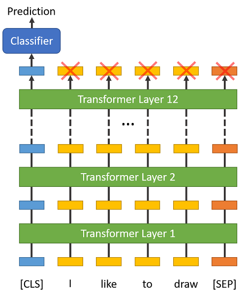
4. bert head#

default BertModel head
BertForMaskedLM

4.1 `BertModel` head vs `BertForMaskedLM`#

两者共享同一个 BERT Encoder（12 层 Transformer），区别在于 Encoder 上面加的”头”不同：

graph TB subgraph BertModel E1[BERT Encoder 12层 Transformer] --> LS[last_hidden_state 每个 token 的 768 维向量] E1 --> PL[Pooler 取 CLS → Linear → Tanh] PL --> PO[pooler_output 1个 768 维句子向量] end subgraph BertForMaskedLM E2[BERT Encoder 12层 Transformer 与上面完全相同的权重] --> LS2[last_hidden_state] LS2 --> MLM[MLM Head Linear 768→30522 + Softmax] MLM --> PRED[每个位置的词表概率分布 预测被 Mask 的词] end

4.1.1 Default `BertModel` head#

就是本笔记一直在用的——pooler（BertPooler）：

1
last_hidden_state (1, 8, 768)
2
        │
3
        ▼ 取 [CLS] 位置
4
   (768,) 向量
5
        │
6
        ▼ Linear(768→768) + Tanh
7
  pooler_output (1, 768)  ← 整个句子的"摘要向量"

作为”基础模型”，BertModel 没有内置任何任务头，只提供一个 pooler 用于获取句子级表示。下游任务（如分类）需要你自己在它上面加分类层。

4.1.2 `BertForMaskedLM`#

在 Encoder 之上加了一个 MLM Head——一个 Linear 层，把每个 token 的 768 维映射到 30522 维（词表大小）：

1
# 伪代码
2
last_hidden_state = bert_encoder(input_ids)   # (batch, seq_len, 768)
3
logits = mlm_head(last_hidden_state)           # (batch, seq_len, 30522)
4
# 对每个位置的预测 = argmax(logits, dim=-1)

这是 BERT 预训练任务之一——随机遮住一些词，让模型预测它们。我们在 02 节中介绍过，并且将在 12 节中深入探索。

4.1.3 与这篇笔记的联系#

本笔记的内容	关联
`outputs['last_hidden_state']`	两者都有，是 Encoder 的输出
`outputs['pooler_output']`	仅 `BertModel` 有，BERT 用它做句子分类（如 NSP）
MLM Head	`BertForMaskedLM` 用 `last_hidden_state` 的每个 token 位置来预测被 Mask 的词，不使用 `pooler_output`

所以，我们目前探索的 pooler_output 只是 BERT 默认的一个”头”，BERT 还可以接不同的头来干不同的事——MLM head 只是其中一个例子，还有 BertForSequenceClassification（分类头）、BertForQuestionAnswering（问答头）等。

💡 可以把 BERT Encoder 想象成”发动机”，pooler、MLM Head、分类头等是不同车型的”车身”——发动机一样，用途不同。

音乐

音乐

1. load model and tokenize#

2. forward and pooler output#

3. from scratch#

3.1 代码分析#

第 1 层：`outputs['last_hidden_state']`#

第 2 层：`[0]` — 取第一个 batch#

第 3 层：`[0, :]` — 取 `[CLS]` token 的向量#

第 4 层：`bert.pooler.dense(...)` — 线性变换#

第 5 层：`bert.pooler.activation(...)` — Tanh 激活#

3.1.6 最终验证#

3.1.7 一句话总结#

4. bert head#

4.1 `BertModel` head vs `BertForMaskedLM`#

4.1.1 Default `BertModel` head#

4.1.2 `BertForMaskedLM`#

4.1.3 与这篇笔记的联系#

文章分享

评论区

音乐

文章目录

音乐

音乐

11_bert_head_pooler_output

1. load model and tokenize#

2. forward and pooler output#

3. from scratch#

3.1 代码分析#

第 1 层：outputs['last_hidden_state']#

第 2 层：[0] — 取第一个 batch#

第 3 层：[0, :] — 取 [CLS] token 的向量#

第 4 层：bert.pooler.dense(...) — 线性变换#

第 5 层：bert.pooler.activation(...) — Tanh 激活#

3.1.6 最终验证#

3.1.7 一句话总结#

4. bert head#

4.1 BertModel head vs BertForMaskedLM#

4.1.1 Default BertModel head#

4.1.2 BertForMaskedLM#

4.1.3 与这篇笔记的联系#

文章分享

评论区

音乐

文章目录

第 1 层：`outputs['last_hidden_state']`#

第 2 层：`[0]` — 取第一个 batch#

第 3 层：`[0, :]` — 取 `[CLS]` token 的向量#

第 4 层：`bert.pooler.dense(...)` — 线性变换#

第 5 层：`bert.pooler.activation(...)` — Tanh 激活#

4.1 `BertModel` head vs `BertForMaskedLM`#

4.1.1 Default `BertModel` head#

4.1.2 `BertForMaskedLM`#