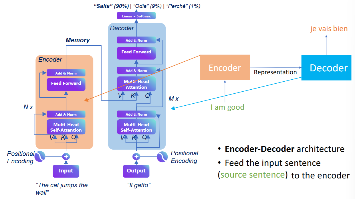
残差连接与层归一化

在 Transformer 的每个编码器和解码器层中，所有子模块（如多头注意力和前馈网络）都被一个 Add & Norm 操作包裹。这个组合是为了保证 Transformer 能够稳定训练。
这个操作由两个部分组成：
- 残差连接 (Add)：该操作将子模块的输入 x 直接加到该子模块的输出 Sublayer(x) 上。这一结构解决了深度神经网络中的梯度消失 (Vanishing Gradients) 问题。在反向传播时，梯度可以绕过子模块直接向前传播，从而保证了即使网络层数很深，模型也能得到有效的训练。其公式可以表示为： $Output=x+Sublayer(x)$ .
- 层归一化 (Norm)：该操作对单个样本的所有特征进行归一化，使其均值为 0 ，方差为 1 。这解决了模型训练过程中的内部协变量偏移 (Internal Covariate Shift) 问题，使每一层的输入分布保持稳定，从而加速模型收敛并提高训练的稳定性。

我们下面从代码层面看看 add&norm 的实现。

0. 初探#

1
import torch
2
from transformers.models.bert import BertModel, BertTokenizer

1
model_name = 'bert-base-uncased'

1
tokenizer = BertTokenizer.from_pretrained(model_name)
2
model = BertModel.from_pretrained(model_name, output_hidden_states=True) # 把每一个 layer 的输出都返回出来

1
model.config

输出为：

1
BertConfig {
2
  "add_cross_attention": false,
3
  "architectures": [
4
    "BertForMaskedLM"
5
  ],
6
  "attention_probs_dropout_prob": 0.1,
7
  "bos_token_id": null,
8
  "classifier_dropout": null,
9
  "dtype": "float32",
10
  "eos_token_id": null,
11
  "gradient_checkpointing": false,
12
  "hidden_act": "gelu",
13
  "hidden_dropout_prob": 0.1,
14
  "hidden_size": 768,
15
  "initializer_range": 0.02,
16
  "intermediate_size": 3072,
17
  "is_decoder": false,
18
  "layer_norm_eps": 1e-12,
19
  "max_position_embeddings": 512,
20
  "model_type": "bert",
21
  "num_attention_heads": 12,
22
  "num_hidden_layers": 12,
23
  "output_hidden_states": true,
24
  "pad_token_id": 0,
25
  "position_embedding_type": "absolute",
26
...
27
  "transformers_version": "5.9.0",
28
  "type_vocab_size": 2,
29
  "use_cache": true,
30
  "vocab_size": 30522
31
}

这里我们需要格外关注 intermediate_size，它指的是 BERT 每层中 Feed-Forward Network（FFN，前馈网络） 的内部扩展维度。

0.1 在 Transformer Encoder 中的位置#

回顾一下 BERT layer 的结构（我们之后也会看到）：

graph LR Input[输入 768维] --> MHA[多头注意力] MHA --> Add1[Add & Norm] Add1 --> FFN[🔶 Feed-Forward Network] FFN --> Add2[Add & Norm] Add2 --> Output[输出 768维]

intermediate_size 就是 FFN 那个橙色块内部的”膨胀宽度”。

0.2 FFN 内部的维度变化#

FFN 由两层全连接网络组成：

1
输入 (768)  ──→  扩展层 (3072)  ──→  压缩层 (768)
2
              W₁(768→3072)        W₂(3072→768)
3
              + GELU激活函数

1
# FFN 的伪代码
2
def feed_forward(x):
3
    # x: (batch, seq_len, 768)
4
    h = x @ W1   # (batch, seq_len, 3072)  ← intermediate_size
5
    h = gelu(h)  # 非线性激活
6
    output = h @ W2  # (batch, seq_len, 768)  回到 hidden_size
7
    return output

0.3 为什么是 3072 = 768 × 4？#

BERT 的 FFN 使用 4 倍扩展的设计：

	BERT-base	通用规律
`hidden_size`	768	$d_{model}$
`intermediate_size`	3072	$4 \times d_{model}$
扩展比	4x	4x

先”膨胀”到 4 倍宽度（给模型更大的容量做非线性变换），再”压缩”回原宽度，这是 Transformer 的标准设计。

0.4 一张图总结#

1
     hidden_size = 768               intermediate_size = 3072
2
    ┌──────────┐                    ┌──────────────────────────────┐
3
    │   词向量  │ ── W₁(768×3072) ──→ │    扩展后的中间表示             │
4
    │   768维  │                    │    3072维                    │
5
    └──────────┘                    └──────────────────────────────┘
6
                                            │ GELU 激活
7
                                            ↓
8
                                    ┌──────────────────────────────┐
9
    ┌──────────┐                    │    非线性变换后的结果           │
10
    │   输出    │ ←── W₂(3072×768) ── │    3072维                    │
11
    │   768维  │                    └──────────────────────────────┘
12
    └──────────┘
13

14
    中间膨胀到 4 倍 → 给模型更大的"思考空间" → 然后压缩回原维度

💡 通俗理解：intermediate_size 就是 FFN 的”肚子”——先把 768 维撑大到 3072 维来充分运算，再缩回 768 维传给下一层。

1
model

输出为：

1
BertModel(
2
  (embeddings): BertEmbeddings(
3
    (word_embeddings): Embedding(30522, 768, padding_idx=0)
4
    (position_embeddings): Embedding(512, 768)
5
    (token_type_embeddings): Embedding(2, 768)
6
    (LayerNorm): LayerNorm((768,), eps=1e-12, elementwise_affine=True, bias=True)
7
    (dropout): Dropout(p=0.1, inplace=False)
8
  )
9
  (encoder): BertEncoder(
10
    (layer): ModuleList(
11
      (0-11): 12 x BertLayer(
12
        (attention): BertAttention(
13
          (self): BertSelfAttention(
14
            (query): Linear(in_features=768, out_features=768, bias=True)
15
            (key): Linear(in_features=768, out_features=768, bias=True)
16
            (value): Linear(in_features=768, out_features=768, bias=True)
17
            (dropout): Dropout(p=0.1, inplace=False)
18
          )
19
          (output): BertSelfOutput(
20
            (dense): Linear(in_features=768, out_features=768, bias=True)
21
            (LayerNorm): LayerNorm((768,), eps=1e-12, elementwise_affine=True, bias=True)
22
            (dropout): Dropout(p=0.1, inplace=False)
23
          )
24
        )
25
        (intermediate): BertIntermediate(
26
...
27
  (pooler): BertPooler(
28
    (dense): Linear(in_features=768, out_features=768, bias=True)
29
    (activation): Tanh()
30
  )
31
)

回顾我们在 03 节中介绍过的关于 BERT 模型的架构，我们知道 BertLayer 的架构如下：

attention: BertAttention
- self: BertSelfAttention
- output: BertSelfOutput
intermediate: BertIntermediate, 768 -> $4\times 768$
output: BertOutput, $4\times 768$ -> 768

再看看我们一开头给出的 Transformer 架构图，实际上：

attention 中的 self 与 output 共同构成了 encoder 中 Multi-Head Attention + Add & Norm 的部分；
而 intermediate 与 output 共同构成了 encoder 中 Feed Forward + Add & Norm 的部分；

MLP

MLP(Multi-Layer Perceptron，多层感知机)就是由多层全连接层（Linear / Dense）堆叠而成的前馈神经网络，每层之间夹一个非线性激活函数。

这里的 intermediate 和 output 实际上是两层 MLP. 我们可以把它们拆开来看：

1
第 1 层: BertIntermediate          第 2 层: BertOutput
2
┌──────────────────────┐      ┌──────────────────────────┐
3
│ Linear(768 → 3072)   │      │ Linear(3072 → 768)        │
4
│        ↓              │      │        ↓                  │
5
│ GELU 激活函数         │      │ Dropout                   │
6
│        ↓              │      │        ↓                  │
7
│ 输出: (batch, 3072)  │ ───→ │ Add (残差: + attention_out)│
8
└──────────────────────┘      │        ↓                  │
9
                              │ LayerNorm                 │
10
                              │        ↓                  │
11
                              │ 输出: (batch, 768)        │
12
                              └──────────────────────────┘

所以：

1
                    MLP（两层）
2
    ┌─────────────────────────────────────────────┐
3
    │                                             │
4
    │  attention_out ──→ Linear(768→3072) ──→ GELU ──→ Linear(3072→768) ──→ ...
5
    │   (输入 x)        ↑  BertIntermediate  ↑         ↑  BertOutput  ↑
6
    │                   └── 第 1 层 ────────┘         └── 第 2 层 ───┘
7
    │                                             │
8
    └─────────────────────────────────────────────┘
9
                            FFN = 两层 MLP

FFN 用两层 MLP 的主要原因是，如果只有一层 Linear(768→768)，那就是一个简单的线性变换，没有任何非线性能力。模型学到的只是输入的线性组合，表达能力很弱。

而如果用 768 -> 3072 -> 768 的两层结构：

先膨胀：768 → 3072，给模型更大的”容量”去学习复杂模式
加非线性：GELU 激活，让模型能学到非线性关系
再压缩：3072 → 768，把信息压缩回原维度，传给下一层

1. model output#

1
test_sentence = 'this is a test sentence'
2

3
model_inputs = tokenizer(test_sentence, return_tensors='pt')

1
model.eval()
2
with torch.no_grad():
3
    outputs = model(**model_inputs)

1
outputs.keys()

输出为：

1
odict_keys(['last_hidden_state', 'pooler_output', 'hidden_states'])

1
outputs[2][0] # embeddings layer

输出为：

1
tensor([[[ 0.1686, -0.2858, -0.3261,  ..., -0.0276,  0.0383,  0.1640],
2
         [-0.6485,  0.6739, -0.0932,  ...,  0.4475,  0.6696,  0.1820],
3
         [-0.6270, -0.0633, -0.3143,  ...,  0.3427,  0.4636,  0.4594],
4
         ...,
5
         [ 0.6010, -0.6970, -0.2001,  ...,  0.2960,  0.2060, -1.7181],
6
         [ 0.8323,  0.2878,  0.0021,  ...,  0.2628, -1.1310, -1.2708],
7
         [-0.1481, -0.2948, -0.1690,  ..., -0.5009,  0.2544, -0.0700]]])

关于 BERT 模型的 outputs，我们在 07 节中进行了详尽的探索，此处不再赘述。总之，outputs[2] 表示的是所有 hidden layers 的输出（包括第 0 层 embedding layer 与 12 个 transformer layers）.

1
outputs[2][1] # first transformer layer

输出为：

1
tensor([[[ 0.1556, -0.0080, -0.0707,  ...,  0.0786,  0.0213,  0.0616],
2
         [-0.5333,  0.5799,  0.1044,  ...,  0.0241,  0.4888,  0.0161],
3
         [-1.0609, -0.3058, -0.5043,  ...,  0.1874,  0.2874,  0.4032],
4
         ...,
5
         [ 0.8206, -0.6656, -0.7054,  ...,  0.1347,  0.1117, -1.9040],
6
         [ 1.1128,  0.6603, -0.1509,  ...,  0.3253, -1.0006, -1.9106],
7
         [-0.0736,  0.0346,  0.0376,  ..., -0.4506,  0.6585, -0.0502]]])

看完了我们获得的结果，下面我们来从零把 BERT layer 串起来。

2. from scratch#

BertLayer
- attention: BertAttention
  - self: BertSelfAttention
  - output: BertSelfOutput
- intermediate: BertIntermediate, 768 -> $4\times 768$
- output: BertOutput, $4\times 768$ -> 768

1
embeddings = outputs[2][0]

1
layer = model.encoder.layer[0]

2.1 第一次 add & norm，发生在 MHA 内部#

1
MHA_output = layer.attention.self(embeddings)
2
MHA_output

输出为：

1
(tensor([[[ 0.2979,  0.0801, -0.0037,  ..., -0.0142,  0.1290,  0.0828],
2
          [ 0.3935,  0.1356, -0.0920,  ...,  0.0211,  0.1677,  0.0011],
3
          [ 0.1696,  0.1449, -0.1039,  ...,  0.1604,  0.2172,  0.0310],
4
          ...,
5
          [-0.0617,  0.1968, -0.0669,  ...,  0.1126,  0.1933, -0.0204],
6
          [-0.2835,  0.1495, -0.0021,  ...,  0.0973,  0.1865, -0.0636],
7
          [ 0.2575,  0.1120, -0.1008,  ...,  0.0175,  0.1508,  0.0878]]],
8
        grad_fn=<ViewBackward0>),
9
 None)

这里的 MHA_output 对应的就是架构图中 encoder 第一个 Multi-Head Self-Attention 的输出。

1
attention_output = layer.attention.output(MHA_output[0], embeddings) # 注意力输出 + 输入的残差连接
2
attention_output

输出为：

1
tensor([[[ 0.6143, -0.2061, -0.5682,  ...,  0.2557,  0.1224,  0.3388],
2
         [-0.6751,  1.0598, -0.2210,  ...,  0.6263,  1.1682,  0.1998],
3
         [-0.5969,  0.1463, -0.5549,  ...,  0.5272,  0.5071,  0.6439],
4
         ...,
5
         [ 1.3291, -1.1190, -0.1960,  ...,  0.6164,  0.4293, -2.4704],
6
         [ 1.8784,  0.5158,  0.1902,  ...,  0.5298, -1.3812, -2.0257],
7
         [ 0.7376, -0.7000, -0.0992,  ..., -0.9356,  0.5831, -0.4610]]],
8
       grad_fn=<NativeLayerNormBackward0>)

MHA_output[0]

MHA_output[0] 实际上是一个 tuple，包含两个元素：

1
MHA_output = layer.attention.self(embeddings)
2

3
# MHA_output = (
4
#     tensor([[...]]),   ← [0] 注意力计算结果，形状 (1, seq_len, 768)
5
#     None               ← [1] 注意力权重矩阵，None 因为没请求
6
# )

这里的 attention_output 就是结构图中经过第一个 Add & Norm 块后的输出。

2.2 第二次 add & norm，发生在 MLP 内部#

1
MLP1 = layer.intermediate(attention_output)
2
MLP1.shape # torch.Size([1, 7, 3072])

1
MLP2 = layer.output(MLP1, attention_output) # MLP 输出 + 输入的残差连接
2
MLP2.shape # torch.Size([1, 7, 768])
3
MLP2

输出为：

1
tensor([[[ 0.1556, -0.0080, -0.0707,  ...,  0.0786,  0.0213,  0.0616],
2
         [-0.5333,  0.5799,  0.1044,  ...,  0.0241,  0.4888,  0.0161],
3
         [-1.0609, -0.3058, -0.5043,  ...,  0.1874,  0.2874,  0.4032],
4
         ...,
5
         [ 0.8206, -0.6656, -0.7054,  ...,  0.1347,  0.1117, -1.9040],
6
         [ 1.1128,  0.6603, -0.1509,  ...,  0.3253, -1.0006, -1.9106],
7
         [-0.0736,  0.0346,  0.0376,  ..., -0.4506,  0.6585, -0.0502]]],
8
       grad_fn=<NativeLayerNormBackward0>)

可以看到这里的结果与之前 outputs[2][1] 的结果是一模一样的。

音乐

音乐

0. 初探#

0.1 在 Transformer Encoder 中的位置#

0.2 FFN 内部的维度变化#

0.3 为什么是 3072 = 768 × 4？#

0.4 一张图总结#

1. model output#

2. from scratch#

2.1 第一次 add & norm，发生在 MHA 内部#

2.2 第二次 add & norm，发生在 MLP 内部#

文章分享

评论区

音乐

文章目录

音乐

音乐

10_add_&_norm_residual_conn

0. 初探#

0.1 在 Transformer Encoder 中的位置#

0.2 FFN 内部的维度变化#

0.3 为什么是 3072 = 768 × 4？#

0.4 一张图总结#

1. model output#

2. from scratch#

2.1 第一次 add & norm，发生在 MHA 内部#

2.2 第二次 add & norm，发生在 MLP 内部#

文章分享

评论区

音乐

文章目录