1
import torch
2
from torch import nn
3
import transformers
4
import numpy as np
5
import pandas as pd
6
import matplotlib.pyplot as plt

1
print(torch.__version__) # 2.6.0+cu124
2
print(transformers.__version__) # 5.9.0

1
import matplotlib as mpl
2
mpl.rcParams["figure.dpi"] = 200 # 默认为 100，设置为 200 可以让图像更清晰

1. text classification#

也叫 sequence classification（text 就是 sequence 的一种）
sentiment analysis
- 情感分析：就是一种文本分类
  - 电商评论
  - social web: weibo/twitter

1.1 emotions 数据集#

1
from datasets import load_dataset

1
emotions = load_dataset("dair-ai/emotion")
2
emotions # dataset Dict

输出为：

1
DatasetDict({
2
    train: Dataset({
3
        features: ['text', 'label'],
4
        num_rows: 16000
5
    })
6
    validation: Dataset({
7
        features: ['text', 'label'],
8
        num_rows: 2000
9
    })
10
    test: Dataset({
11
        features: ['text', 'label'],
12
        num_rows: 2000
13
    })
14
})

可见，在默认设置下，会自动分为三块数据集：训练集、测试集和验证集，比例为 8:1:1. 此外，数据集为一个字典类型。

1
emotions.keys() # dict_keys(['train', 'validation', 'test'])

1
print(emotions['train']), type(emotions['train']) # 数据集结构概览
2
# 继续支持 key
3
print(emotions['train']['text'][:5]) # 前五条文本数据
4
print(emotions['train']['label'][:5]) # 前五条标签数据
5
# 支持 index
6
print(emotions['train'][:5]) # 前五条数据，包含文本和标签

输出为：

1
Dataset({
2
    features: ['text', 'label'],
3
    num_rows: 16000
4
})
5

6
['i didnt feel humiliated', 'i can go from feeling so hopeless to so damned hopeful just from being around someone who cares and is awake', 'im grabbing a minute to post i feel greedy wrong', 'i am ever feeling nostalgic about the fireplace i will know that it is still on the property', 'i am feeling grouchy']
7
[0, 0, 3, 2, 3]
8

9
{'text': ['i didnt feel humiliated', 'i can go from feeling so hopeless to so damned hopeful just from being around someone who cares and is awake', 'im grabbing a minute to post i feel greedy wrong', 'i am ever feeling nostalgic about the fireplace i will know that it is still on the property', 'i am feeling grouchy'], 'label': [0, 0, 3, 2, 3]}

这里的 [0, 0, 3, 2, 3] 是每条文本对应的情感分类标签（数字编码）。emotions 数据集有 6 类情感：

标签值	情感
0	sadness（悲伤）
1	joy（快乐）
2	love（喜爱）
3	anger（愤怒）
4	fear（恐惧）
5	surprise（惊讶）

所以前 5 条分别是：sadness、sadness、anger、love、anger.

1
print(emotions['train'].features) # 查看所有特征
2

3
print(emotions['train'].features['label']) # 查看标签特征
4

5
print(emotions['train'].features['label'].int2str(2)) # 查看标签数字 2 对应的字符串标签

输出为：

1
{'text': Value('string'), 'label': ClassLabel(names=['sadness', 'joy', 'love', 'anger', 'fear', 'surprise'])}
2

3
ClassLabel(names=['sadness', 'joy', 'love', 'anger', 'fear', 'surprise'])
4

5
love

第一行：这里我们可以从第一行输出看到，训练集有两个特征：

特征	类型	说明
`text`	`Value('string')`	文本内容，字符串类型
`label`	`ClassLabel(names=[...])`	分类标签，有 6 个类别名称

第二行：可以看到 label 是一个 ClassLabel 类型，内部维护了数字到情感名称的映射：

数字	情感
0	sadness（悲伤）
1	joy（快乐）
2	love（喜爱）
3	anger（愤怒）
4	fear（恐惧）
5	surprise（惊讶）

第 3 行：int2str() 是 ClassLabel 提供的方法，功能是将数字标签转换为对应的文字。这里传入 2，返回 "love".

对应的还有反向方法 str2int()，例如：

1
emotions['train'].features['label'].str2int('love')  # 返回 2

1
labels = emotions['train'].features['label'].names
2
print(labels) # 标签列表
3

4
num_classes = len(labels)
5
print(num_classes) # 标签数量

输出为：

1
['sadness', 'joy', 'love', 'anger', 'fear', 'surprise']
2

3
6

这里我们把六类标签都提取出来，方便后面分析。

1.2 data visualization analysis#

dataset -> dataframe
text length
label freq

1.2.1 dataset to dataframe#

1
emotions_df = pd.DataFrame.from_dict(emotions['train'])

这里我们将 HuggingFace 中的 Dataset 转化成了 pandas 库中的 DataFrame. 因为 Hugging Face 的 Dataset 虽然功能强大，但在数据分析和可视化方面不如 pandas 方便，而 DataFrame 提供了大量便捷的方法。

1
print(emotions_df.shape, emotions_df.columns) # 数据集形状和列名
2
emotions_df[:5] # 前五行数据

输出为：

1
(16000, 2) Index(['text', 'label'], dtype='str')
2

3

4
                 text                                label
5
0  i didnt feel humiliated                              0
6
1  i can go from feeling so hopeless to so damned...  0
7
2  im grabbing a minute to post i feel greedy wrong  3
8
3  i am ever feeling nostalgic about the fireplac...  2
9
4  i am feeling grouchy                              3

1
emotions_df['label_name'] = emotions_df['label'].apply(lambda x: emotions['train'].features['label'].int2str(x))
2
emotions_df[:5] # 前五行数据，包含标签名称

输出为：

1
          text                                   label  label_name
2
0  i didnt feel humiliated                              0  sadness
3
1  i can go from feeling so hopeless to so damned...  0  sadness
4
2  im grabbing a minute to post i feel greedy wrong  3  anger
5
3  i am ever feeling nostalgic about the fireplac...  2  love
6
4  i am feeling grouchy                              3  anger

1.2.2 label analysis#

1
emotions_df.label.value_counts()

输出为：

1
label
2
1    5362
3
0    4666
4
3    2159
5
4    1937
6
2    1304
7
5     572
8
Name: count, dtype: int64

这是训练集中的标签分布，所有加起来恰好为 16000 条样本。

1
emotions_df.label_name.value_counts()

输出为：

1
label_name
2
joy         5362
3
sadness     4666
4
anger       2159
5
fear        1937
6
love        1304
7
surprise     572
8
Name: count, dtype: int64

1
plt.figure(figsize=(4,3))
2
emotions_df.label_name.value_counts().plot(kind='bar')
3
plt.xlabel('Label')
4
plt.ylabel('Count')
5
plt.title('Distribution of Labels')
6
plt.xticks(rotation=45)
7
plt.show()

输出如下图：

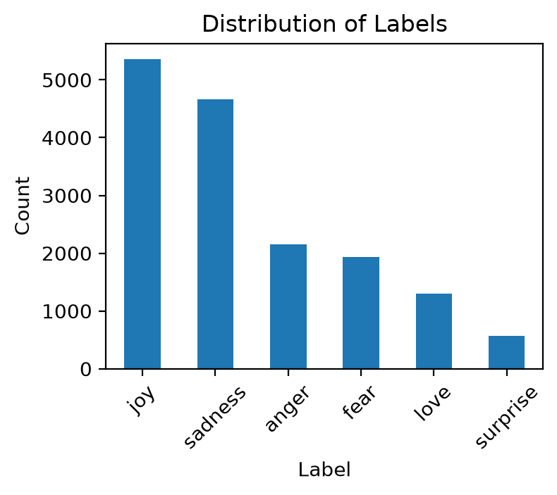
1.2.3 text length analysis#

1
plt.figure(figsize=(4,3))
2
emotions_df['word per tweet'] = emotions_df['text'].str.split().apply(len)
3
emotions_df.boxplot(
4
    column='word per tweet',
5
    by='label_name',
6
    grid=False,
7
    color='blue'
8
    # showfliers=False
9
)
10
plt.suptitle('')
11
plt.xlabel('')

输出如下图：

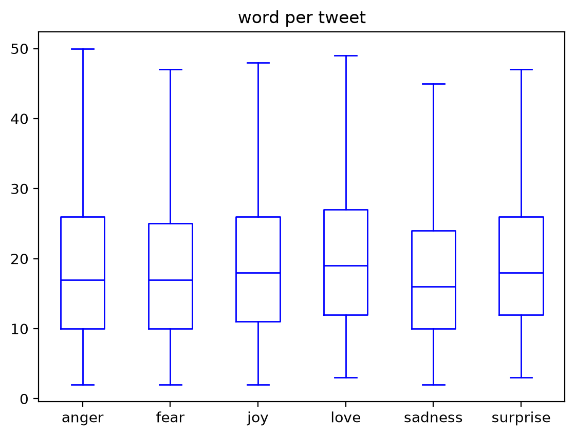
这里我们使用箱线图（Boxplot）进行分析，它展示了 emotion 数据集中，不同情感标签（怒、惧、喜、爱、悲、惊）的推文文本长度（单词数）的分布情况。

我们主要看以下几个关键元素：

横轴 (X 轴)：表示不同的分类标签（如 anger, fear, joy 等）。
纵轴 (Y 轴)：表示推文的单词数量（word per tweet）。
蓝色的矩形箱体 (Box)：
- 中间的横线：表示中位数 (Median)。将该类别下所有推文的长度从小到大排列后，排在最中间的那个长度值。例如，所有类别推文长度的中位数都在 15-20 个单词左右。
- 箱子的顶边：表示上四分位数 (75th Percentile)。有 75% 的推文长度小于这个值。
- 箱子的底边：表示下四分位数 (25th Percentile)。有 25% 的推文长度小于这个值。
- 箱子的高度：表示四分位距 (IQR)，包含了中间 50% 数据所在的范围，反映了数据的集中程度。
上下延伸的线段 (Whiskers, “胡须”)：
- 表示数据的范围（不包含异常值）。通常延伸到 $1.5 \times IQR$ 内的最极值。
- 顶端的横线是最大值（非异常值情况下的最大长度）。
- 底端的横线是最小值（非异常值情况下的最小长度）。可以看到所有类别的最小词数都在 2 个左右。
异常值 (Outliers)：在代码中，你设置了 showfliers=False，这意味着这幅图隐藏了离群点（异常长或异常短的极端个例），从而让主体分布更加清晰。

从这幅图中可以得出的结论：

不同情感的推文长度分布非常相似，中位数大多在 15-20 词之间。
各个情感类别的绝大多数推文（约 75%）长度都在 30 个单词以内，最长的（不计极端异常值）在 45-50 个单词左右。
这表明各种情感表达在句子长度上并没有明显的差异偏好。这对于后续使用 Transformer 模型（比如 BERT，它有最大序列长度限制，如 512，这取决于 Token 数量而非单词，但通过单词数可以看出通常比较短，不太会被截断）进行文本分类是一个有用的参考信息。

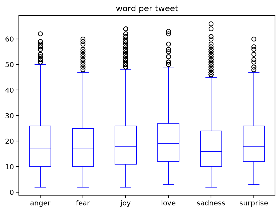
当我们把 showfliers=False 注解掉后，就会看到有一些异常点。

回顾一下箱线图的知识：

正常范围（胡须的范围）：箱线图有一条规则用来界定什么是“正常”的数据范围。通常，程序会计算一个叫做 四分位距（IQR，即上四分位数减去下四分位数，也就是蓝色箱子的高度） 的值。
- 上方的胡须最高会延伸到：上四分位数 + $1.5 \times IQR$ 。
- 超过这个界限的数据点，就会被判定为异常值。
异常点的意义：在这个特定的数据集中，这些小黑圈代表个别极其冗长的推文。
- 绝大部分推文长度都在 50 个单词（上方的蓝色横线）以内。
- 但有少数人在推文中写了 50~70 多个单词甚至更多（图中的黑圈最高达到了接近 70）。
- 这些非常长的句子不符合大众的发推习惯，所以被当做异常点单独画在上面。

对我们做深度学习/自然语言处理的启示

当我们把文本输入给 BERT 模型时，BERT 有一个最大长度限制（往往设为 128、256 或 512）。看到最高的黑圈也就是 70 左右的> 单词数，我们就可以很放心地把模型最大序列长度（max_length）截断设得比较小（比如 128），因为即使是这些“异常”的超长文 > 本，也完全能被容纳，不会因为被截断而丢失关键信息。

1
print(emotions_df['word per tweet'].max()) # 最长文本的单词数量
2
print(emotions_df['word per tweet'].idxmax()) # 最长文本的索引

输出为：

可以看到，训练集中最长文本的索引就是第 6322 条数据，共有 66 个单词。

1
print(emotions_df.iloc[6322]) # 查看第 6322 条数据
2
emotions_df.iloc[6322]['text'] # 查看第 6322 条数据的文本内容

输出为：

1
text              i guess which meant or so i assume no photos n...
2
label                                                             0
3
label_name                                                  sadness
4
word per tweet                                                   66
5
Name: 6322, dtype: object
6

7
'i guess which meant or so i assume no photos no words or no other way to convey what it really feels unless you feels it yourself or khi bi t au th m i bi t th ng ng i b au i rephrase it to a bit more gloomy context unless you are hurt yourself you will never have sympathy for the hurt ones'

这里我们使用到了 iloc 方法。iloc 是 pandas 中基于整数位置（integer-location）的索引方法，用于按行号（从 0 开始）访问 DataFrame 或 Series 中的数据。

它的核心特点如下：

方法	基于	示例	说明
`iloc`	整数位置（行号）	`df.iloc[0]`	第 0 行
`loc`	标签/索引名	`df.loc[0]`	索引为 0 的行（可能不是第一行）
`[]`	列名	`df['text']`	获取列

iloc vs loc 对比如下：

1
# iloc —— 按行号（不考虑索引值）
2
emotions_df.iloc[0]     # 无论索引是什么，取第 0 行
3

4
# loc —— 按索引标签（不考虑位置）
5
emotions_df.loc[0]      # 取索引值等于 0 的行

当 DataFrame 的索引是默认的 0, 1, 2, ... 时，两者结果相同。但如果索引被重置或乱序，它们就不同了：

1
df = pd.DataFrame({'a': [10, 20, 30]}, index=[2, 0, 1])
2
df.iloc[0]  # 返回索引为 2 的行：a=10 （第 0 个位置）
3
df.loc[0]   # 返回索引为 0 的行：a=20 （标签为 0）

在这里，因为 DataFrame 使用的是默认整数索引，所以 iloc[6322] 和 loc[6322] 结果一样，但 iloc 的语义更明确——就是按行号取数据。

1
print(emotions_df['word per tweet'].min()) # 最短文本的单词数量
2
print(emotions_df['word per tweet'].idxmin()) # 最短文本的索引

输出为：

可以看到，训练集中最短文本的索引就是第 4150 条数据，只有 2 个单词。

1
print(emotions_df.iloc[4150]) # 查看第 4150 条数据
2
emotions_df.iloc[4150]['text'] # 查看第 4150 条数据的文本内容

输出为：

1
text              earth crake
2
label                       4
3
label_name               fear
4
word per tweet              2
5
Name: 4150, dtype: object
6

7
'earth crake'

1.3 text -> tokens#

数据集转化为模型接受的输入类型：

Subword Tokenization
- WordPiece
  - BERT and DistilBERT
HuggingFace
- ~/.cache/huggingface/
- model config
  - tokenizer.model_max_length
  - tokenizer.model_input_names

我们接下来要做的就是——将原始文本转换为模型能理解的输入格式。

1.3.1 tokenizer#

1
from transformers import AutoTokenizer

1
model_ckpt = 'distilbert-base-uncased'
2
tokenizer = AutoTokenizer.from_pretrained(model_ckpt)

这里的模型名称也包含一些信息 distilbert-base-uncased：

base 表示模型大小，有 medium， large ，我们这里选用的是 base 大小；
uncased 表示对大小写不敏感，或者说，就是小写的意思，表示这个模型在训练时将所有文本转换为小写。

1
print(tokenizer.encode('hello world')) # 编码文本为 token id 列表
2
print(tokenizer.encode('HELLO WORLD')) # 编码文本为 token id 列表，注意大写会被转换为小写
3
print(tokenizer.encode('Hello World'))

输出为：

1
[101, 7592, 2088, 102]
2
[101, 7592, 2088, 102]
3
[101, 7592, 2088, 102]

可以看到，转化出来的 token id 都是相同的。

1
tokenizer.encode(emotions_df.iloc[6322]['text']) # 编码第 6322 条数据的文本内容为 token id 列表

输出为：

注意这里以 [CLS] 开头，[SEP] 结束。

1
print(tokenizer.vocab_size) # 查看 tokenizer 的词汇表大小
2
print(tokenizer.model_max_length) # 查看 tokenizer 的最大输入长度
3
print(tokenizer.model_input_names) # 查看 tokenizer 的输入名称列表

输出为：

1
30522
2
512
3
['input_ids', 'token_type_ids', 'attention_mask']

1
for special_id in tokenizer.all_special_ids:
2
    print(special_id, tokenizer.decode(special_id)) # 查看特殊 token 的 id 和对应的字符串

输出为：

1
100 [UNK]
2
102 [SEP]
3
0 [PAD]
4
101 [CLS]
5
103 [MASK]

这部分在前面我们探索 BERT 模型时已经进行了详尽的介绍，这里不再赘述。

1.3.2 tokenize the whole dataset#

1
def batch_tokenize(batch):
2
    return tokenizer(batch['text'], padding=True, truncation=True)

1
emotions_encoded = emotions.map(batch_tokenize, batched=True, batch_size=None)

1
emotions_encoded

输出为：

1
DatasetDict({
2
    train: Dataset({
3
        features: ['text', 'label', 'input_ids', 'token_type_ids', 'attention_mask'],
4
        num_rows: 16000
5
    })
6
    validation: Dataset({
7
        features: ['text', 'label', 'input_ids', 'token_type_ids', 'attention_mask'],
8
        num_rows: 2000
9
    })
10
    test: Dataset({
11
        features: ['text', 'label', 'input_ids', 'token_type_ids', 'attention_mask'],
12
        num_rows: 2000
13
    })
14
})

可以看到，经过 tokenize 的数据集除了原来的 text 和 label 之外，还多出了 input_ids, token_type_ids, attention_mask.

1
batch_tokenize(emotions['train'][:5]) # 批量编码前五条数据的文本内容

输出为：

1
{'input_ids': [[101, 1045, 2134, 2102, 2514, 26608, 102, 0, 0, 0, 0, 0, 0, 0, 0, 0, 0, 0, 0, 0, 0, 0, 0], [101, 1045, 2064, 2175, 2013, 3110, 2061, 20625, 2000, 2061, 9636, 17772, 2074, 2013, 2108, 2105, 2619, 2040, 14977, 1998, 2003, 8300, 102], [101, 10047, 9775, 1037, 3371, 2000, 2695, 1045, 2514, 20505, 3308, 102, 0, 0, 0, 0, 0, 0, 0, 0, 0, 0, 0], [101, 1045, 2572, 2412, 3110, 16839, 9080, 12863, 2055, 1996, 13788, 1045, 2097, 2113, 2008, 2009, 2003, 2145, 2006, 1996, 3200, 102, 0], [101, 1045, 2572, 3110, 24665, 7140, 11714, 102, 0, 0, 0, 0, 0, 0, 0, 0, 0, 0, 0, 0, 0, 0, 0]], 'token_type_ids': [[0, 0, 0, 0, 0, 0, 0, 0, 0, 0, 0, 0, 0, 0, 0, 0, 0, 0, 0, 0, 0, 0, 0], [0, 0, 0, 0, 0, 0, 0, 0, 0, 0, 0, 0, 0, 0, 0, 0, 0, 0, 0, 0, 0, 0, 0], [0, 0, 0, 0, 0, 0, 0, 0, 0, 0, 0, 0, 0, 0, 0, 0, 0, 0, 0, 0, 0, 0, 0], [0, 0, 0, 0, 0, 0, 0, 0, 0, 0, 0, 0, 0, 0, 0, 0, 0, 0, 0, 0, 0, 0, 0], [0, 0, 0, 0, 0, 0, 0, 0, 0, 0, 0, 0, 0, 0, 0, 0, 0, 0, 0, 0, 0, 0, 0]], 'attention_mask': [[1, 1, 1, 1, 1, 1, 1, 0, 0, 0, 0, 0, 0, 0, 0, 0, 0, 0, 0, 0, 0, 0, 0], [1, 1, 1, 1, 1, 1, 1, 1, 1, 1, 1, 1, 1, 1, 1, 1, 1, 1, 1, 1, 1, 1, 1], [1, 1, 1, 1, 1, 1, 1, 1, 1, 1, 1, 1, 0, 0, 0, 0, 0, 0, 0, 0, 0, 0, 0], [1, 1, 1, 1, 1, 1, 1, 1, 1, 1, 1, 1, 1, 1, 1, 1, 1, 1, 1, 1, 1, 1, 0], [1, 1, 1, 1, 1, 1, 1, 1, 0, 0, 0, 0, 0, 0, 0, 0, 0, 0, 0, 0, 0, 0, 0]]}

这里就是简单看一下具体编码出来的东西，还记得我们之前在 batch_tokenize 函数中设置了 padding=True.

1
print(type(emotions_encoded['train']['input_ids'])) # 查看编码后的输入 id 的数据类型
2
emotions_encoded['train']['input_ids'][:3] # 查看编码后的输入 id 列表的前 3 条数据

输出为：

1
datasets.arrow_dataset.Column
2

3
[[101,
4
  1045,
5
  2134,
6
  2102,
7
  2514,
8
  26608,
9
  102,
10
  0,
11
...
12
  0,
13
  0,
14
  0,
15
  0,
16
  0]]

这里的 Column 是 Hugging Face dataset 库中基于 Apache Arrow 格式的一种列式数据结构，可以简单地看作是一个增强版的 list：

它的外部接口兼容 list，使用起来与 list 一样；
内部存储用 Arrow，兼顾了易用性和高性能。

1
emotions_encoded.set_format(type='torch', columns=['input_ids', 'attention_mask', 'label']) # 设置数据集格式为 PyTorch，指定需要返回的列

1
print(type(emotions_encoded['train']['input_ids'])) # 查看编码后的输入 id 的数据类型
2
print(type(emotions_encoded['train'][0]['input_ids'])) # 取单行
3
print(type(emotions_encoded['train'][:5]['input_ids'])) # 取多行

输出为：

1
<class 'datasets.arrow_dataset.Column'>
2
<class 'torch.Tensor'>
3
<class 'torch.Tensor'>

这里需要注意的是，set_format 只在我们 取行（样本） 时生效，而不是在取整列时生效。

这是因为 set_format 主要是为了配合 PyTorch 的 DataLoader 使用——DataLoader 按行（样本）逐个取数据，而不是按列取。

2. fine-tune transformers#

2.1 distilbert-base-uncased#

DistilBERT 是 BERT 的精简版（蒸馏版），通过**知识蒸馏（Knowledge Distillation）**技术训练得到。

核心区别：

对比项	BERT-base	DistilBERT
参数量	~110M	~66M（减少 40%）
层数（Transformer blocks）	12 层	6 层（减半）
推理速度	基准	快约 60%
性能（准确率）	基准	保留约 97% 的性能
模型大小（磁盘）	~440MB	~260MB

如何实现的？

DistilBERT 使用 知识蒸馏 三步走：

1
1. 训练好一个大的 BERT（Teacher 模型）
2
2. DistilBERT（Student 模型）复制 Teacher 的中间层的一半
3
3. Student 学习模仿 Teacher 的输出分布，而不仅仅是 ground truth 标签

关键点：

层数减半：6 层 vs 12 层（DistilBERT 每 2 层对应 BERT 的 1 层）
去掉了 Token Type IDs：DistilBERT 不支持 token_type_ids（因为蒸馏时去掉了下一句预测任务）
保留了核心能力：仍支持 Masked LM，仍可用于分类、QA、NER 等任务

一句话总结：

DistilBERT ≈ BERT 的 “轻量版”——体积小 40%、速度快 60%、性能只下降约 3%，非常适合资源受限的场景或对推理延迟有要求的应用。

1
from transformers import AutoModel
2

3
model_ckpt = 'distilbert-base-uncased'
4
model = AutoModel.from_pretrained(model_ckpt)
5
model # 模型结构概览

输出为：

1
DistilBertModel(
2
  (embeddings): Embeddings(
3
    (word_embeddings): Embedding(30522, 768, padding_idx=0)
4
    (position_embeddings): Embedding(512, 768)
5
    (LayerNorm): LayerNorm((768,), eps=1e-12, elementwise_affine=True)
6
    (dropout): Dropout(p=0.1, inplace=False)
7
  )
8
  (transformer): Transformer(
9
    (layer): ModuleList(
10
      (0-5): 6 x TransformerBlock(
11
        (attention): DistilBertSelfAttention(
12
          (q_lin): Linear(in_features=768, out_features=768, bias=True)
13
          (k_lin): Linear(in_features=768, out_features=768, bias=True)
14
          (v_lin): Linear(in_features=768, out_features=768, bias=True)
15
          (out_lin): Linear(in_features=768, out_features=768, bias=True)
16
          (dropout): Dropout(p=0.1, inplace=False)
17
        )
18
        (sa_layer_norm): LayerNorm((768,), eps=1e-12, elementwise_affine=True)
19
        (ffn): FFN(
20
          (dropout): Dropout(p=0.1, inplace=False)
21
          (lin1): Linear(in_features=768, out_features=3072, bias=True)
22
          (lin2): Linear(in_features=3072, out_features=768, bias=True)
23
          (activation): GELUActivation()
24
        )
25
        (output_layer_norm): LayerNorm((768,), eps=1e-12, elementwise_affine=True)
26
      )
27
    )
28
  )
29
)

这里我们可以看到 DistilBERT 模型的整体架构：

2.1.1 DistilBERT 整体架构概览#

1
DistilBertModel
2
├── Embeddings（嵌入层）
3
└── Transformer（Transformer 层）
4
    └── 6 × TransformerBlock
5
        ├── Attention（多头自注意力）
6
        ├── sa_layer_norm（注意力后的 LayerNorm）
7
        └── FFN（前馈神经网络）
8
            └── output_layer_norm（FFN 后的 LayerNorm）

1️⃣ Embeddings（嵌入层）#

1
Embeddings(
2
  (word_embeddings):       Embedding(30522, 768)     ← 词嵌入
3
  (position_embeddings):   Embedding(512, 768)       ← 位置嵌入
4
  (LayerNorm):             LayerNorm(768)            ← 层归一化
5
  (dropout):               Dropout(p=0.1)            ← 随机失活
6
)

组件	参数	说明
`word_embeddings`	30522 × 768	词汇表大小 30522，每个词映射为 768 维向量
`position_embeddings`	512 × 768	最大序列长度 512，每个位置一个 768 维向量
`LayerNorm`	768	层归一化，稳定训练
`Dropout`	p=0.1	10% 的神经元随机丢弃，防止过拟合

注意：与 BERT 不同，DistilBERT 没有 token_type_ids（片段嵌入），因为蒸馏时去掉了下一句预测任务。

2️⃣ Transformer（6 层 TransformerBlock）#

1
(0-5): 6 x TransformerBlock

BERT-base 有 12 层，DistilBERT 精简为 6 层，每层由 Attention + FFN 组成。

Attention（多头自注意力）#

1
DistilBertSelfAttention(
2
  (q_lin):     Linear(768 → 768)   ← Query 投影
3
  (k_lin):     Linear(768 → 768)   ← Key 投影
4
  (v_lin):     Linear(768 → 768)   ← Value 投影
5
  (out_lin):   Linear(768 → 768)   ← 输出投影
6
  (dropout):   Dropout(p=0.1)
7
)

输入维度：768（每个 token 的隐藏状态）
输出维度：768
多头注意力：q/k/v 的维度 768 会被拆分为多个注意力头（通常是 12 头，每头 64 维）
计算流程： $Attention(Q, K, V) = \text{softmax}\left(\frac{QK^T}{\sqrt{d_k}}\right)V$
out_lin 将多头结果拼接后投影回 768 维

`sa_layer_norm`（注意力后的层归一化）#

1
LayerNorm(768)

在残差连接之后进行归一化。这是 DistilBERT 的标准化设计——先 Attention，再加残差，最后 LayerNorm。

FFN（前馈神经网络）#

1
FFN(
2
  (lin1):       Linear(768 → 3072)    ← 升维 4 倍
3
  (activation): GELUActivation()       ← 激活函数
4
  (lin2):       Linear(3072 → 768)    ← 降维回 768
5
  (dropout):    Dropout(p=0.1)
6
)

两层线性层，中间是一个扩张-收缩结构：
- lin1：768 → 3072（扩大 4 倍）
- GELU 激活函数（高斯误差线性单元，比 ReLU 更平滑）
- lin2：3072 → 768（压缩回原始维度）
这种结构让模型能在更高维空间中学习复杂的特征交互

`output_layer_norm`#

1
LayerNorm(768)

与 Attention 一样，在 FFN 的残差连接之后再进行一次归一化。

2.1.2 单层 TransformerBlock 的数据流#

1
输入 (768)
2
    ↓
3
  ┌──────────────────────┐
4
  │  Self-Attention      │
5
  │  Q/K/V 投影 + 多头计算 │
6
  └────────┬─────────────┘
7
    ↓ (残差连接)
8
  + 输入
9
    ↓
10
  LayerNorm (sa_layer_norm)
11
    ↓
12
  ┌──────────────────────┐
13
  │  FFN                 │
14
  │  768 → 3072 → 768    │
15
  └────────┬─────────────┘
16
    ↓ (残差连接)
17
  + 输入
18
    ↓
19
  LayerNorm (output_layer_norm)
20
    ↓
21
 输出 (768) → 进入下一层

2.1.3 与 BERT-base 的架构差异总结#

组件	BERT-base (12 层)	DistilBERT (6 层)
嵌入层	word + position + token_type	word + position (无 token_type)
每层结构	Attention → LayerNorm → FFN → LayerNorm	(残差后) LayerNorm → Attention → LayerNorm → FFN
注意力头数	12 头	12 头
隐藏维度	768	768
激活函数	GELU	GELU

架构上的主要区别是 LayerNorm 的位置——DistilBERT 将 LayerNorm 移到了残差连接之后（Post-LN 的变体），这是一种更稳定的设计选择。

1
from transformer_utils import get_params

1
# 查看模型参数总数
2
get_params(model) # np.int64(66362880)

1
from transformers import AutoModel
2

3
model_ckpt = 'bert-base-uncased'
4
model = AutoModel.from_pretrained(model_ckpt)
5
get_params(model) # np.int64(109482240)

可以看到，distilbert-base-uncased 仅有 6 千万参数量；而我们之前频繁接触的 bert-base-uncased 有超过 1 亿参数量。

1
model

输出为：

1
BertModel(
2
  (embeddings): BertEmbeddings(
3
    (word_embeddings): Embedding(30522, 768, padding_idx=0)
4
    (position_embeddings): Embedding(512, 768)
5
    (token_type_embeddings): Embedding(2, 768)
6
    (LayerNorm): LayerNorm((768,), eps=1e-12, elementwise_affine=True)
7
    (dropout): Dropout(p=0.1, inplace=False)
8
  )
9
  (encoder): BertEncoder(
10
    (layer): ModuleList(
11
      (0-11): 12 x BertLayer(
12
        (attention): BertAttention(
13
          (self): BertSelfAttention(
14
            (query): Linear(in_features=768, out_features=768, bias=True)
15
            (key): Linear(in_features=768, out_features=768, bias=True)
16
            (value): Linear(in_features=768, out_features=768, bias=True)
17
            (dropout): Dropout(p=0.1, inplace=False)
18
          )
19
          (output): BertSelfOutput(
20
            (dense): Linear(in_features=768, out_features=768, bias=True)
21
            (LayerNorm): LayerNorm((768,), eps=1e-12, elementwise_affine=True)
22
            (dropout): Dropout(p=0.1, inplace=False)
23
          )
24
        )
25
        (intermediate): BertIntermediate(
26
          (dense): Linear(in_features=768, out_features=3072, bias=True)
27
          (intermediate_act_fn): GELUActivation()
28
        )
29
        (output): BertOutput(
30
          (dense): Linear(in_features=3072, out_features=768, bias=True)
31
          (LayerNorm): LayerNorm((768,), eps=1e-12, elementwise_affine=True)
32
          (dropout): Dropout(p=0.1, inplace=False)
33
        )
34
      )
35
    )
36
  )
37
  (pooler): BertPooler(
38
    (dense): Linear(in_features=768, out_features=768, bias=True)
39
    (activation): Tanh()
40
  )
41
)

BERT 模型的结构我们在之前的章节中已经介绍地非常具体了，二者模型的架构也在前面进行了详尽的对比，这里仅做回顾。

1
from transformers import AutoModelForSequenceClassification
2

3
model_ckpt = 'distilbert-base-uncased'
4
device = torch.device('cuda' if torch.cuda.is_available() else 'cpu')
5
model = AutoModelForSequenceClassification.from_pretrained(model_ckpt, num_labels=num_classes).to(device)
6
model

输出为：

1
DistilBertForSequenceClassification(
2
  (distilbert): DistilBertModel(
3
    (embeddings): Embeddings(
4
      (word_embeddings): Embedding(30522, 768, padding_idx=0)
5
      (position_embeddings): Embedding(512, 768)
6
      (LayerNorm): LayerNorm((768,), eps=1e-12, elementwise_affine=True)
7
      (dropout): Dropout(p=0.1, inplace=False)
8
    )
9
    (transformer): Transformer(
10
      (layer): ModuleList(
11
        (0-5): 6 x TransformerBlock(
12
          (attention): DistilBertSelfAttention(
13
            (q_lin): Linear(in_features=768, out_features=768, bias=True)
14
            (k_lin): Linear(in_features=768, out_features=768, bias=True)
15
            (v_lin): Linear(in_features=768, out_features=768, bias=True)
16
            (out_lin): Linear(in_features=768, out_features=768, bias=True)
17
            (dropout): Dropout(p=0.1, inplace=False)
18
          )
19
          (sa_layer_norm): LayerNorm((768,), eps=1e-12, elementwise_affine=True)
20
          (ffn): FFN(
21
            (dropout): Dropout(p=0.1, inplace=False)
22
            (lin1): Linear(in_features=768, out_features=3072, bias=True)
23
            (lin2): Linear(in_features=3072, out_features=768, bias=True)
24
            (activation): GELUActivation()
25
          )
26
          (output_layer_norm): LayerNorm((768,), eps=1e-12, elementwise_affine=True)
27
        )
28
      )
29
    )
30
  )
31
  (pre_classifier): Linear(in_features=768, out_features=768, bias=True)
32
  (classifier): Linear(in_features=768, out_features=6, bias=True)
33
  (dropout): Dropout(p=0.2, inplace=False)
34
)

2.1.4 `DistilBertModel` vs `DistilBertForSequenceClassification`#

仔细观察输出，核心区别在于 分类头（Classification Head） 的添加：

1
DistilBertModel                                   DistilBertForSequenceClassification
2
│                                                 │
3
├── Embeddings                                    ├── Embeddings（完全相同）
4
│   ├── word_embeddings (30522, 768)              │   ├── word_embeddings (30522, 768)
5
│   ├── position_embeddings (512, 768)            │   ├── position_embeddings (512, 768)
6
│   ├── LayerNorm(768)                            │   ├── LayerNorm(768)
7
│   └── Dropout(p=0.1)                            │   └── Dropout(p=0.1)
8
│                                                 │
9
├── Transformer (6层)     ← 完全相同 →            ├── Transformer (6层)
10
│                                                 │
11
│                                  ⭐ 多出的部分：│
12
│                                                 ├── pre_classifier: Linear(768→768)
13
│                                                 ├── dropout: Dropout(p=0.2)  ← 注意：0.2
14
│                                                 └── classifier: Linear(768→6)

新增的三个组件详解#

1
(pre_classifier): Linear(in_features=768, out_features=768, bias=True)
2
(dropout):       Dropout(p=0.2, inplace=False)
3
(classifier):    Linear(in_features=768, out_features=6, bias=True)

组件	维度变化	作用
`pre_classifier`	768 → 768	额外的线性变换层，在分类前做一次特征映射，增加模型表达能力
`Dropout(p=0.2)`	—	20% 随机失活，比 base 模型的 0.1 更高，因为分类头容易过拟合
`classifier`	768 → 6	最终分类层，将 768 维隐层状态映射到 6 类情感得分

这里需要注意的是，如果我们没有传入 num_labels=num_classes 参数，那么默认设置为 2 个分类头：

1
  (pre_classifier): Linear(in_features=768, out_features=768, bias=True)
2
  (classifier): Linear(in_features=768, out_features=2, bias=True)
3
  (dropout): Dropout(p=0.2, inplace=False)

而传入 num_labels=num_classes 后，根据我们前面计算的结果，num_classes=6，所以模型就有了 6 个分类头。

数据流对比#

1
DistilBertModel (基础模型):
2
输入 → Embeddings → 6层 Transformer → [CLS]位置的768维向量
3

4
DistilBertForSequenceClassification (分类模型):
5
输入 → Embeddings → 6层 Transformer → [CLS]位置的768维向量
6
                                          ↓
7
                                    pre_classifier (768→768)
8
                                          ↓
9
                                       ReLU 激活
10
                                          ↓
11
                                    Dropout(p=0.2)
12
                                          ↓
13
                                    classifier (768→6)
14
                                          ↓
15
                                    6 类情感得分 (logits)

关键点：

DistilBertModel 输出的是所有 token 位置的完整 768 维隐层状态（[batch_size, seq_len, 768]），你需要自己取 [CLS] 并添加分类层
DistilBertForSequenceClassification 已经内置了分类头，自动取 [CLS] token 的输出经过分类头，直接输出 6 类情感得分（[batch_size, 6]），可以直接用 CrossEntropyLoss 训练

一句话总结：

DistilBertForSequenceClassification = DistilBertModel + 分类头。base 模型只负责提取特征，ForSequenceClassification 在顶部额外挂了 pre_classifier → Dropout → classifier 三层，让你可以直接做分类任务。

在运行完上述代码后，此时如果我们用 nvidia-smi 查看显卡状态，会发现模型已经加载到了显存中。

此外，还要注意上述代码的另一段输出：

1
Loading weights: 100%|██████████| 100/100 [00:00<00:00, 16317.71it/s]
2
[transformers] [1mDistilBertForSequenceClassification LOAD REPORT[0m from: distilbert-base-uncased
3
Key                     | Status     |
4
------------------------+------------+-
5
vocab_transform.bias    | UNEXPECTED |
6
vocab_layer_norm.bias   | UNEXPECTED |
7
vocab_projector.bias    | UNEXPECTED |
8
vocab_layer_norm.weight | UNEXPECTED |
9
vocab_transform.weight  | UNEXPECTED |
10
pre_classifier.weight   | MISSING    |
11
classifier.weight       | MISSING    |
12
classifier.bias         | MISSING    |
13
pre_classifier.bias     | MISSING    |
14

15
Notes:
16
- UNEXPECTED:  can be ignored when loading from different task/architecture; not ok if you expect identical arch.
17
- MISSING:  those params were newly initialized because missing from the checkpoint. Consider training on your downstream task.

这里我们会发现，pre_classifier.weight, classifier.weight, classifier.bias 和 pre_classifier.bias 参数是没有被正确初始化的。换句话说，它们目前只是一些随机值。要想用 DistilBertForSequenceClassification 这个模型去做预测，我们需要在自己的下游任务中训练这个模型，以 fine-tune 这部分数值。

2.2 trainer#

1
from huggingface_hub import notebook_login
2

3
notebook_login()

1
from transformers import TrainingArguments, Trainer

1
batch_size = 64
2
logging_steps = len(emotions_encoded['train']) // batch_size
3
model_name = f'{model_ckpt}-finetuned-emotion-classification'
4
training_args = TrainingArguments(
5
    output_dir=model_name,
6
    learning_rate=2e-5,
7
    num_train_epochs=4,
8
    per_device_train_batch_size=batch_size,
9
    per_device_eval_batch_size=batch_size,
10
    eval_strategy='epoch',
11
    weight_decay=0.01,
12
    disable_tqdm=False,
13
    logging_steps=logging_steps,
14
    push_to_hub=True,
15
    log_level='error'
16
)

我们来简单介绍一下上面的几个参数：

eval_strategy='epoch' ：评估策略；

控制什么时候在验证集上评估模型。

⚠️ 注意：在 transformers 5.x 版本中，这个参数已从 evaluation_strategy 重命名为 eval_strategy。如果用了旧名字会报错 unexpected keyword argument。

取值	含义
`'no'`	训练期间不评估
`'steps'`	每 `eval_steps` 步评估一次
`'epoch'`	每个 epoch 结束后评估一次 ✅ 最常用

设置为 'epoch' 意味着每个 epoch 跑完后，模型会自动在验证集上计算损失和准确率，这样你就可以看到每个 epoch 的训练损失和验证损失，判断模型是否过拟合。

weight_decay=0.01 ：权重衰减；

权重衰减是一种 正则化技术，也叫 L2 正则化。它的核心思想是：在每次更新参数时，让权重向零方向稍微缩小一点点，防止模型过度依赖某些特征。

数学原理

标准梯度下降更新公式：

$w_{t+1} = w_t - \eta \cdot \nabla L(w_t)$

加入权重衰减后：

$w_{t+1} = w_t - \eta \cdot (\nabla L(w_t) + \lambda \cdot w_t)$

展开：

$w_{t+1} = w_t - \eta \cdot \nabla L(w_t) - \eta \lambda \cdot w_t$

$w_{t+1} = (1 - \eta\lambda) \cdot w_t - \eta \cdot \nabla L(w_t)$

可以看到，权重 $w_t$ 在更新前先被乘以一个小于 1 的系数 $(1 - \eta\lambda)$ ，这就是”衰减”的含义。

想象你在画一条曲线来拟合一些数据点。如果没有权重衰减，你可能会为了让曲线穿过每一个点而把曲线画得弯弯曲曲、剧烈抖动（过拟合）。权重衰减就像给曲线加了一个”弹性约束”——让曲线尽量平滑、简单，不要过度扭曲。

一些直觉理解：

过拟合的模型往往权重值很大、很极端（对某些特征过度敏感）
权重衰减惩罚大权重，迫使权重保持较小的值
小权重意味着模型对每个特征的依赖更均衡，不会因为某个特征而做出极端判断

实际效果：

✅ 防止过拟合
✅ 提高泛化能力
✅ 在 NLP 任务中几乎总是有益的
⚠️ 值太大（如 0.1）会导致欠拟合；值太小（如 0.0001）几乎没效果
0.01 是一个比较常用且合理的值

disable_tqdm=False ：显示进度条；

logging_steps=logging_steps ：日志输出步长；

控制每隔多少个训练步输出一次日志（损失值、学习率等）。

在我们的设置中，训练集有 16000 条数据，每批 64 条，所以每个 epoch 有 250 步。 因此 logging_steps=250 意味着每训练完一个 epoch 输出一次日志。

关于如何选择合适的值：

场景	`logging_steps` 建议
想看每步的损失变化	较小值，如 `10` 或 `50`
只想看每个 epoch 的概况	`len(train_dataset) // batch_size`（即每 epoch 一次）
训练很快（几分钟）	小一些，可以看到损失下降曲线
训练很慢（几小时）	大一些，避免日志太多刷屏

log_level='error' ：日志级别；

控制 Hugging Face Transformers 库本身输出的日志详细程度。

日志级别金字塔：

1
                    ╔═══════════════╗
2
                    ║   CRITICAL    ║  ← 最严重，程序可能崩溃
3
                    ╠═══════════════╣
4
                    ║    ERROR      ║  ← 发生了错误但程序还能继续
5
                    ╠═══════════════╣
6
                    ║    WARNING    ║  ← ⭐ 默认级别，潜在问题提醒
7
                    ╠═══════════════╣
8
                    ║     INFO      ║  ← 一般信息（模型加载、保存等）
9
                    ╠═══════════════╣
10
                    ║    DEBUG      ║  ← 最详细，调试用
11
                    └───────────────┘

设置的含义：

`log_level`	显示的信息	举例
`'debug'`	全部信息	最详细的调试输出
`'info'`	info 及以上	”Loading model…” “Saving checkpoint…”
`'warning'`	warning 及以上	”Some weights are not used” ⭐ 默认
`'error'`	仅 error	只有真正的错误才显示
`'critical'`	仅 critical	几乎什么都不显示

在我们的场景下，log_level='error' 说明：

这意味着 Transformers 库内部的所有信息、警告都被抑制了
只有真正的错误才会打印出来
这样做的好处是输出更干净，不会被一大堆 “Some weights of the model checkpoint were not used…” 之类的警告刷屏

关于其他训练设置：

trainer 默认自动开启 torch 的多 gpu 模式；
- per_device_train_batch_size 设定每个 GPU 上的样本数量；
- 一般而言，多 GPU 模式希望多个 GPU 的性能尽量接近，否则多 GPU 的速度将由最慢的 GPU 决定；
per_device_eval_batch_size 类似；
learning_rate 以及 weight_decay 默认采用 AdamW 的优化算法。

1
from transformer_utils import compute_classification_metrics
2

3
trainer = Trainer(
4
    model=model,
5
    args=training_args,
6
    train_dataset=emotions_encoded['train'],
7
    eval_dataset=emotions_encoded['validation'],
8
    compute_metrics=compute_classification_metrics
9
)

1
trainer.train()

输出为：

1
TrainOutput(global_step=1000, training_loss=0.31053504371643065, metrics={'train_runtime': 123.707, 'train_samples_per_second': 517.352, 'train_steps_per_second': 8.084, 'total_flos': 1440685723392000.0, 'train_loss': 0.31053504371643065, 'epoch': 4.0})

上面就是 Hugging Face Trainer 训练完成后输出的训练报告，包含了三个主要部分：

1
TrainOutput(
2
    global_step=1000,                                            # ① 总步数
3
    training_loss=0.31053504371643065,                           # ② 训练损失
4
    metrics={...}                                                # ③ 详细指标字典
5
)

global_step=1000 — 总训练步数

$\text{总步数} = \text{训练集样本数} \times \text{epoch数} \div batch\_size$

$= 16,000 \times 4 \div 64 = 1,000$

training_loss=0.3105 — 平均训练损失

损失函数（Loss） 衡量的是模型预测与真实标签之间的差距。

$\text{Loss} = -\frac{1}{N}\sum_{i=1}^{N}\sum_{c=1}^{C} y_{i,c} \log(p_{i,c})$

这是交叉熵损失（Cross-Entropy Loss），多分类任务的标配：

损失值	含义
~2.0 以上	模型几乎在瞎猜（6 类随机猜 ≈ log6 ≈ 1.79）
~1.0	模型开始学到一些规律
~0.31（我们的值）	✅ 模型学到了很强的规律
~0.0	完美拟合（也要小心过拟合）

从开始时的较高损失下降到 0.31，说明模型收敛得很好。

metrics — 详细指标

训练用时：

指标	值	解读
`train_runtime`	123.7 秒（约 2 分钟）	训练总耗时
`train_samples_per_second`	517.35 条/秒	每秒处理 517 条文本
`train_steps_per_second`	8.08 步/秒	每秒更新 8 次参数

这里使用的设备是单张 RTX4080 laptop.

总计算量：

指标	值	解读
`total_flos`	1.44 × 10¹⁵ FLOPs	浮点运算总数

FLOPs（Floating Point Operations）：衡量计算量的单位。这个数字的意思是——整个训练过程一共执行了约 1.4 千万亿次浮点运算。

最终损失：

指标	值
`train_loss`	0.3105（和上面的 `training_loss` 一样）

一张图总结：

flowchart LR subgraph 输入 A["16000 条推文 6 类情感"] end subgraph 训练配置 B["DistilBERT 66M 参数"] C["Batch = 64 Epoch = 4"] D["总步数 = 1000"] end subgraph 结果 E["训练损失: 0.31 耗时: 2 分钟"] end A --> B --> C --> D --> E

1
preds_output = trainer.predict(emotions_encoded['validation'])
2
preds_output

输出为：

1
PredictionOutput(predictions=array([[ 5.302656  , -1.1895534 , -1.4358829 , -1.5534474 , -1.7579308 ,
2
        -1.9462327 ],
3
       [ 5.2939024 , -1.075267  , -2.0208688 , -1.311696  , -1.3683631 ,
4
        -1.9535345 ],
5
       [-1.6112493 ,  2.7801807 ,  3.1485417 , -1.6580076 , -2.5439014 ,
6
        -2.3933396 ],
7
       ...,
8
       [-1.6095595 ,  5.4891787 , -0.56173605, -1.5967947 , -2.361022  ,
9
        -1.9980701 ],
10
       [-2.050608  ,  3.349502  ,  3.0134823 , -1.7501646 , -2.6897838 ,
11
        -2.3941755 ],
12
       [-1.664848  ,  5.413096  , -0.7544189 , -2.052569  , -2.1643562 ,
13
        -1.0560712 ]], shape=(2000, 6), dtype=float32), label_ids=array([0, 0, 2, ..., 1, 1, 1], shape=(2000,)), metrics={'test_loss': 0.14947177469730377, 'test_accuracy': 0.934, 'test_precision': 0.9347108725250716, 'test_recall': 0.934, 'test_f1': 0.934171624082316, 'test_runtime': 1.3177, 'test_samples_per_second': 1517.783, 'test_steps_per_second': 24.285})

上面就是 trainer.predict() 在 验证集（2000 条样本）上的输出，它的结构如下：

1
PredictionOutput(
2
    predictions=...,    # ① 模型输出的原始分数（logits）
3
    label_ids=...,      # ② 真实标签
4
    metrics=...         # ③ 评估指标
5
)

predictions ：模型输出的原始分数。

形状为 (2000, 6)，即 2000 条样本 × 6 类情感，每个值叫做 logit（logits）——也就是 softmax 之前的原始分数。

看前几条数据：

1
样本1: [ 5.30, -1.19, -1.44, -1.55, -1.76, -1.95]  → 类别 0 (sadness) 得分最高 ✅
2
样本2: [ 5.29, -1.08, -2.02, -1.31, -1.37, -1.95]  → 类别 0 (sadness) 得分最高 ✅
3
样本3: [-1.61,  2.78,  3.15, -1.66, -2.54, -2.39]  → 类别 2 (love) 得分最高 ✅

Logits 如何变成预测结果？

$\text{softmax}(z_i) = \frac{e^{z_i}}{\sum_{j=1}^{6} e^{z_j}} \quad\rightarrow\quad \text{argmax} \rightarrow \text{最终类别}$

1
# compute_classification_metrics 中正是这样做的
2
preds = pred.predictions.argmax(-1)   # 取每行最大值所在的索引 → 预测类别

原始 logits	softmax 后	argmax（预测类别）
[5.30, -1.19, -1.44, …]	[0.998, 0.0003, 0.0002, …]	0 (sadness) ✅
[-1.61, 2.78, 3.15, …]	[0.006, 0.407, 0.574, …]	2 (love) ✅

label_ids ：真实标签

1
array([0, 0, 2, ..., 1, 1, 1], shape=(2000,))

对应 6 类情感：

数字	情感
0	sadness
1	joy
2	love
3	anger
4	fear
5	surprise

metrics ：评估指标 + 核心结果

总体性能：

指标	值	含义
`test_loss`	0.1495	验证集上的损失，比训练损失 0.31 还低，说明模型泛化很好
`test_accuracy`	0.934 (93.4%)	准确率——2000 条中正确预测了约 1868 条
`test_precision`	0.9347	精确率（加权平均）
`test_recall`	0.9340	召回率（加权平均）
`test_f1`	0.9342	F1 分数（精确率和召回率的调和平均）

四个指标都接近 93.4%，说明模型在各类情感上表现均衡，没有对某些类别特别偏袒或歧视。

推理性能：

指标	值	含义
`test_runtime`	1.32 秒	评估 2000 条只用了 1.3 秒
`test_samples_per_second`	1517.78 条/秒	每秒处理约 1500 条推文
`test_steps_per_second`	24.29 步/秒	每秒执行约 24 步

相比训练时每秒 517 条，推理速度快了 3 倍（因为推理不需要反向传播计算梯度）。

一张图总结：

flowchart TD subgraph 输入 A["验证集 2000 条推文"] end subgraph 模型推理 B["DistilBERT → 6 类 logits (2000 × 6)"] end subgraph 后处理 C["softmax → 概率分布"] D["argmax → 预测类别"] end subgraph 对比 E["预测类别 vs 真实标签"] end subgraph 结果 F["✅ 准确率 93.4% ✅ F1 分数 93.4% ✅ 仅用 1.3 秒"] end A --> B --> C --> D --> E --> F

1
preds_output = trainer.predict(emotions_encoded['validation'])
2
y_preds = np.argmax(preds_output.predictions, axis=-1)

这里我们就是提取预测结果中的类别，其中：

trainer.predict() 返回一个 PredictionOutput 对象，包含三个部分：

1
PredictionOutput(
2
    predictions=array(shape=(2000, 6)),   # ← 每条样本对 6 类情感的原始得分 (logits)
3
    label_ids=array(shape=(2000,)),       # ← 每条样本的真实标签 (0~5)
4
    metrics={...}                          # ← 评估指标
5
)

np.argmax() 就是沿着最后一个维度（6 类情感）找出得分最高的索引。
- predictions 的形状如上所示，为 (2000, 6)，每一行是这条样本对 6 类情感的得分。

1
y_true = emotions_encoded['validation']['label']

这里我们从预处理好的验证集中提取 真实标签列。

1
# import importlib
2
# import transformer_utils
3
# importlib.reload(transformer_utils)

1
from transformer_utils import plot_confusion_matrix

1
plot_confusion_matrix(y_true, y_preds, labels=labels)

输出如下图：

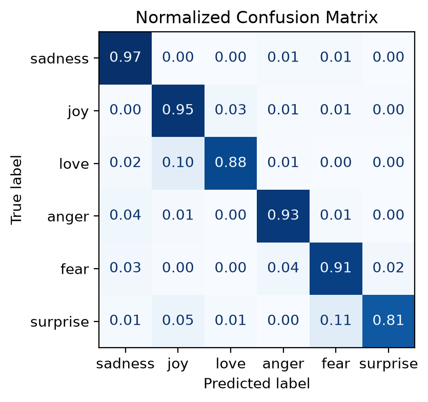
从输出的混淆矩阵可以看出：

97% 的 sadness 被正确预测；
- 分别有 1% 的 sadness 被错误预测为了 anger 和 fear.
95% 的 joy 被正确预测；
93% 的 anger 被正确预测；
91% 的 fear 被正确预测；
88% 的 love 被正确预测；
81% 的 surprise 被正确预测；

下面我们来看测试集的结果。

1
preds_output = trainer.predict(emotions_encoded['test'])
2
y_preds = np.argmax(preds_output.predictions, axis=-1)
3
y_true = emotions_encoded['test']['label']
4
plot_confusion_matrix(y_true, y_preds, labels=labels)

输出结果如下图：

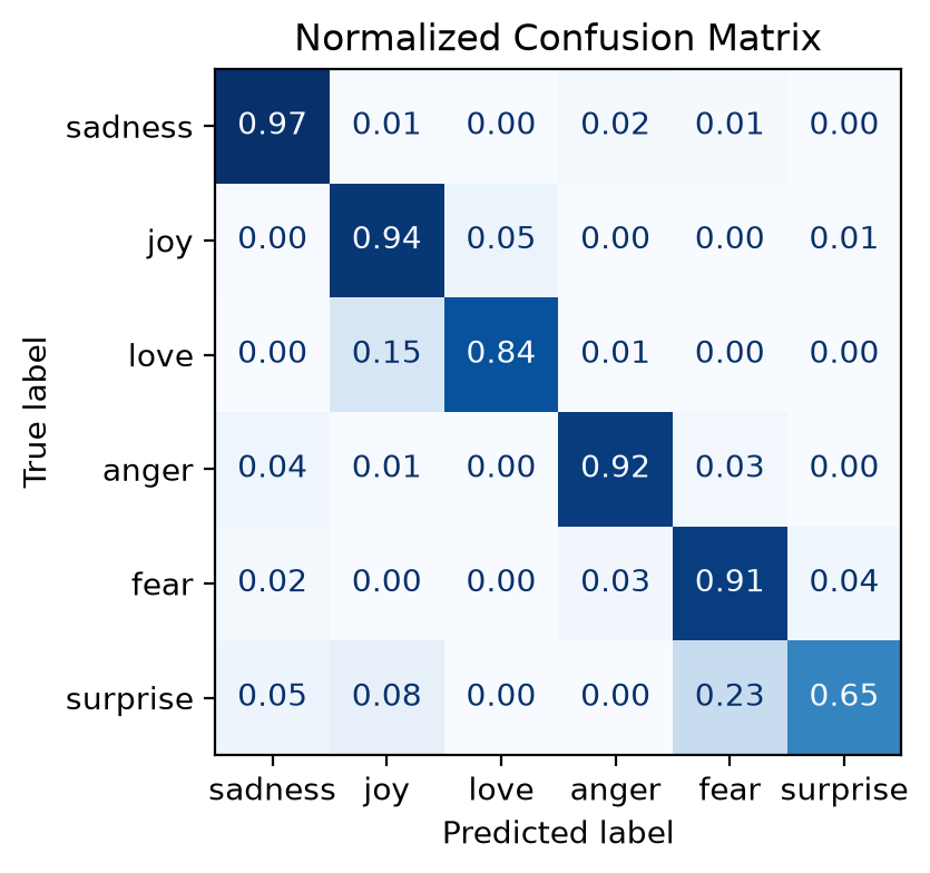
可以看到，在测试集上，模型在区分 surprise 和 fear 时表现较差，有 23% 的 surprise 都被错误归类为了 fear.

3. result analysis#

1
from torch.nn.functional import cross_entropy

1
tokenizer.model_input_names

1
def forward_pass_with_label(batch):
2
    # 将输入数据移动到设备上，并过滤出模型需要的输入
3
    inputs = {k: v.to(device) for k, v in batch.items() if k in tokenizer.model_input_names}
4
    with torch.no_grad():
5
        outputs = model(**inputs)
6
        pred_label = torch.argmax(outputs.logits, dim=-1)
7
        loss = cross_entropy(outputs.logits, batch['label'].to(device), reduction='none')
8
    # 将 loss 和 pred_label 从 GPU 移动到 CPU，并转换为 numpy 数组返回
9
    return {'loss': loss.cpu().numpy(), 'pred_label': pred_label.cpu().numpy()}

这个函数的目的是对每一条样本单独计算损失，而非对整个 batch 求平均：

1
inputs = {k: v.to(device) for k, v in batch.items() if k in tokenizer.model_input_names}

遍历 batch 中的所有字段，即 ['text', 'label', 'input_ids', 'token_type_ids', 'attention_mask', 'loss', 'pred_label']；
只保留 tokenizer.model_input_names 中的字段，即 ['input_ids', 'token_type_ids', 'attention_mask']，排除 label 和 text 等非模型输入字段；
将所有选中的输入移到 GPU 上，即 device.

1
with torch.no_grad():
2
        outputs = model(**inputs)
3
        pred_label = torch.argmax(outputs.logits, dim=-1)
4
        loss = cross_entropy(outputs.logits, batch['label'].to(device), reduction='none')

这里是很经典的前向传播过程了，因此这里只重点介绍一下 cross_entropy 的参数：

outputs.logits ：预测，形状为 (batch_size, 6)，原始的 logits
batch['label'].to(device) ：真实的标签，形状为 (batch_size,)，每个值 0-5.
- 要注意的是因为我们前面是在 GPU 上创建了 inputs，而此时 batch 还在 CPU 上，PyTorch 要求参与计算的张量必须在同一个设备上，所以我们这里要将 batch['label'] 移动到 GPU.
reduction='none' ：表示不对 batch 求 mean，而是返回每个样本独立的 loss，形状从 () 变为 (batch_size,).
- 默认情形下，reduction='mean'，即把一个 batch 中所有样本的损失平均成一个数。

1
return {'loss': loss.cpu().numpy(), 'pred_label': pred_label.cpu().numpy()}

将 GPU 上的张量移回 CPU，否则 HuggingFace Dataset 无法存储；
转为 numpy 数组，便于后续分析和可视化；
返回一个字典，包含两个字段：loss 和 pred_label.

1
emotions_encoded['validation'] = emotions_encoded['validation'].map(
2
    forward_pass_with_label, batched=True, batch_size=16)

通过 map 将 forward_pass_with_label 应用到整个验证集上。这样，验证集的每条样本都多了两个新字段：

loss ：该样本的损失；
pred_label ：模型预测的类别。

1
emotions_encoded['validation']

输出为：

1
Dataset({
2
    features: ['text', 'label', 'input_ids', 'token_type_ids', 'attention_mask', 'loss', 'pred_label'],
3
    num_rows: 2000
4
})

可以看到，现在验证集中确实多出了两个新字段。

1
selected_cols = ['text', 'label', 'loss', 'pred_label']

1
emotions_encoded.reset_format()
2
valid_df = pd.DataFrame.from_dict(
3
    {
4
        'text': emotions_encoded['validation']['text'],
5
        'label': emotions_encoded['validation']['label'],
6
        'pred_label': emotions_encoded['validation']['pred_label'],
7
        'loss': emotions_encoded['validation']['loss']
8
    }
9
)
10
valid_df['label'] = valid_df['label'].apply(lambda x: labels[x])
11
valid_df['pred_label'] = valid_df['pred_label'].apply(lambda x: labels[x])

1
valid_df

输出为：

1
                        text                          label  pred_label  loss
2
0  im feeling quite sad and sorry for myself but ...  sadness  sadness      0.005036
3
1  i feel like i am still looking at a blank canv...  sadness  sadness      0.005398
4
2  i feel like a faithful servant                      love  love      0.340381
5
3  i am just feeling cranky and blue                  anger  anger      0.006064
6
4  i can have for a treat or if i am feeling festive  joy      joy          0.004903
7
...  ...  ...  ...  ...
8
1995  im having ssa examination tomorrow in the morn...  sadness  sadness  0.006089
9
1996  i constantly worry about their fight against n...  joy      joy      0.005474
10
1997  i feel its important to share this info for th...  joy      joy      0.004890
11
1998  i truly feel that if you are passionate enough...  joy      joy      0.575697
12
1999  i feel like i just wanna buy any cute make up ...  joy      joy      0.006726
13

14
2000 rows × 4 columns

1
valid_df[valid_df['label'] != valid_df['pred_label']]

输出为：

1
                       text                              label  pred_label  loss
2
17  i know what it feels like he stressed glaring ...      anger  sadness      2.504660
3
27  i feel as if i am the beloved preparing hersel...      joy      love      1.369006
4
35  i am feeling very blessed today that they shar...      joy      love      0.834904
5
60  i miss our talks our cuddling our kissing and ...      love  joy          0.946954
6
91  i feel like the people i know are really gener...      joy      love      0.953229
7
...  ...  ...  ...  ...
8
1958  i so desperately want to be able to help but i...  fear  sadness      0.850377
9
1963  i called myself pro life and voted for perry w...  joy      sadness      5.088876
10
1964  i feel vaguely cheated and a little amused          joy      anger      4.081220
11
1981  i spent a lot of time feeling overwhelmed with...  fear  surprise  0.746432
12
1990  i just feel too overwhelmed i can t see the fo...  fear  surprise  0.984590
13

14
130 rows × 4 columns

这里输出的就是验证集上所有预测错误的样本，总共 130 条。

1
# most labels incorrectly
2
valid_df[valid_df['label'] != valid_df['pred_label']].label.value_counts()

输出为：

1
label
2
joy         38
3
love        22
4
fear        20
5
anger       18
6
sadness     17
7
surprise    15
8
Name: count, dtype: int64

我们可以查看分类错误的样本里的内部分布。

1
valid_df.sort_values(by='loss', ascending=False).head(10)

输出为：

1
                          text                              label      pred_label  loss
2
1500  i guess we would naturally feel a sense of lon...      anger      sadness      6.607152
3
1950  i as representative of everything thats wrong ...      surprise  sadness      6.467403
4
1111  im lazy my characters fall into categories of ...      joy          fear      6.427592
5
1509  i guess this is a memoir so it feels like that...      joy          fear      6.364819
6
882      i feel badly about reneging on my commitment t...      love      sadness      6.108779
7
1963  i called myself pro life and voted for perry w...      joy          sadness      5.088876
8
1840  id let you kill it now but as a matter of fact...      joy          fear      5.073016
9
318      i felt ashamed of these feelings and was scare...      fear      sadness      4.791914
10
405      i have been feeling extraordinarily indecisive...      fear      joy          4.677145
11
1836  i got a very nasty electrical shock when i was...      fear      anger      4.654828

可以打印出 loss 最高的前 10 条样本。

我们可以举其中一个例子：

1
valid_df.iloc[882].text

输出为：

1
'i feel badly about reneging on my commitment to bring donuts to the faithful at holy family catholic church in columbus ohio'

中文翻译过来就是：“我为自己食言，没有给俄亥俄州哥伦布市圣家天主教堂的信徒们带甜甜圈而感到愧疚。”

你发现了吗？这其实是一个标记错误的数据，数据集中给它的 label 是 love，但显然，这句话并不是 love，因此模型预测的 sadness 反而是对的。

对于 dair-ai/emotion 这个数据集而言，它的数据来自于推文，一般的标注流程是：

flowchart LR A["采集推文"] --> B["分发给多个标注者"] B --> C["标注者 A: love"] B --> D["标注者 B: joy"] B --> E["标注者 C: sadness"] C & D & E --> F["取多数投票 或随机选择一个"] F --> G["最终标签: love"]

由于情感标注本身就具有主观性，加之推文是 脱离上下文 被标注的，所以不同的标注者很有可能做出不同的标注。实际上，在学术数据集中，“噪声标签” 是普遍存在的。

所以，我们之前看到的模型 93.4% 的准确率，有一部分”错误”其实是标注本身的歧义造成的——模型可能在某些样本上才是”正确”的。

而通过 loss 排序，我们可以快速发现这些可疑的标注。因为模型在数据中的规律（而非噪声）上收敛，当遇到一个违背规律的标注时，它的 loss 就会异常高。

1
# less loss -> more confident
2
valid_df.sort_values('loss', ascending=True).head(10)

输出为：

1
                          text                          label  pred_label  loss
2
1310  i feel like an ungrateful asshole                  sadness  sadness      0.004158
3
702      i only find out that they are looking and feel...  joy      joy          0.004176
4
21      i feel try to tell me im ungrateful tell me im...  sadness  sadness      0.004195
5
845      i already feel very glamorous have a great day...  joy      joy          0.004204
6
1601  i feel so ungrateful when thinking saying thes...  sadness  sadness      0.004205
7
1502  i feel ungrateful for stupid shit like              sadness  sadness      0.004215
8
212      i own the brushes are constantly used and i fe...  joy      joy          0.004218
9
578      i got to christmas feeling positive about the ...  joy      joy          0.004222
10
1466  i feel so ungrateful to be wishing this pregna...  sadness  sadness      0.004224
11
133      i and feel quite ungrateful for it but i m loo...  sadness  sadness      0.004237

我们再来看升序的情况。可以发现，模型对预测 joy 和 sadness 非常自信

4. to huggingface hub#

1
# 1. 设置标签映射到模型 config 中
2
id2label = {0: 'sadness', 1: 'joy', 2: 'love', 3: 'anger', 4: 'fear', 5: 'surprise'}
3
label2id = {v: k for k, v in id2label.items()}
4
model.config.id2label = id2label
5
model.config.label2id = label2id
6

7
# 2. 推送 tokenizer（包含标签映射）
8
Hug_name = "" # 替换为你的 Hugging Face Hub 用户名
9
tokenizer.push_to_hub(f"{Hug_name}/distilbert-base-uncased-finetuned-emotion-classification")
10

11
# 3. 强制重新推送模型权重
12
trainer.push_to_hub(commit_message="Fix: add id2label and re-upload fine-tuned weights")

这里我们就是将微调好的模型推送到 HuggingFace Hub 上：

flowchart LR A["本地训练好的模型 distilbert-base-uncased- finetuned-emotion- classification"] --> B["打包模型权重 + 配置"] B --> C["上传到 Hugging Face Hub"] C --> D["https://huggingface.co/ 你的用户名/ distilbert-base-uncased- finetuned-emotion- classification"]

我们上传的内容包括：

pytorch_model.bin — 模型权重（66M 参数的数值）
config.json — 模型配置（6 分类、隐藏层维度等）
tokenizer.json / vocab.txt — 分词器文件

上传后，任何人都可以以类似下面的方式加载我们的模型：

1
from transformers import pipeline
2

3
# 就像从官网加载 distilbert 一样
4
classifier = pipeline(
5
    "text-classification",
6
    model="你的用户名/distilbert-base-uncased-finetuned-emotion-classification"
7
)
8

9
classifier("I feel so happy today!")
10
# [{'label': 'joy', 'score': 0.99}]

我们在下面给出了示例，加载你刚刚上传到 HuggingFace 的模型直接用于推理：

1
# hide_output
2
from transformers import pipeline
3

4
# 清除缓存后重新加载
5
import shutil
6
cache_dir = "C:\\Users\\HP\\.cache\\huggingface\\hub\\models--hac1224--distilbert-base-uncased-finetuned-emotion-classification"
7
shutil.rmtree(cache_dir, ignore_errors=True)
8

9
# 创建 classifier
10
classifier = pipeline(
11
    "text-classification",
12
    model="hac1224/distilbert-base-uncased-finetuned-emotion-classification"
13
)

pipeline 会自动帮你完成这些步骤：

加载模型，相当于 AutoModelForSequenceClassification.from_pretrained(...)；
加载分词器，相当于 AutoTokenizer.from_pretrained(...)；
文本编码，相当于 tokenizer(text, padding=True, truncation=True)；
模型推理，相当于 model(**inputs)；
后处理，相当于 softmax -> argmax -> 映射标签名；

通过 classifier 创建一个分类器后，我们之后就可以像这样使用了：

1
classifier("I feel so happy today!")
2
# 输出: [{'label': 'joy', 'score': 0.998}]

它会自动：

从 Hub 下载模型权重和分词器
对输入文本进行分词
用模型推理得到 logits
通过 softmax 计算概率
返回 label（标签名）和 score（置信度）

所以，pipline = 模型 + 分词器 + 预处理 + 后处理的”一键打包”，我们不需要手写任何预处理或后处理代码，输入文本直接出结果。

1
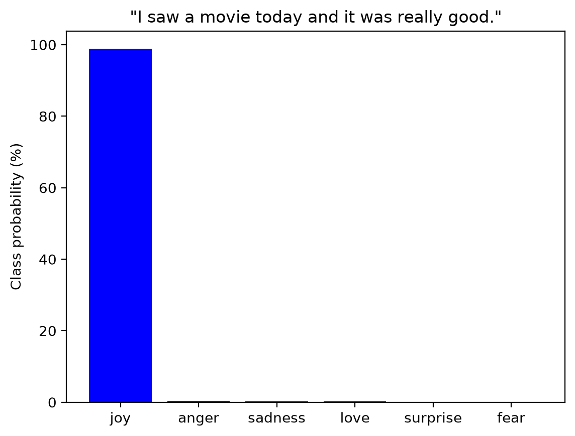
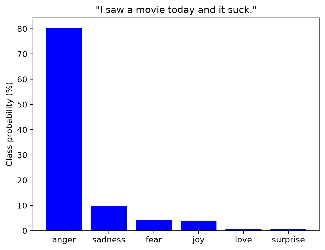
# custom_tweet = 'I saw a movie today and it was really good.'
2
custom_tweet = 'I saw a movie today and it suck.'
3
preds = classifier(custom_tweet, top_k=None)
4
preds

输出为（top_k=None 返回全部 6 类的概率）：

1
# 第一句话的输出
2
[{'label': 'joy', 'score': 0.9890854954719543},
3
 {'label': 'anger', 'score': 0.003720962442457676},
4
 {'label': 'sadness', 'score': 0.002655301010236144},
5
 {'label': 'love', 'score': 0.002034853445366025},
6
 {'label': 'surprise', 'score': 0.0015041438164189458},
7
 {'label': 'fear', 'score': 0.0009992503328248858}]
8

9
# 第二句话的输出
10
[{'label': 'anger', 'score': 0.8032434582710266},
11
 {'label': 'sadness', 'score': 0.09835370630025864},
12
 {'label': 'fear', 'score': 0.04329225793480873},
13
 {'label': 'joy', 'score': 0.040239084511995316},
14
 {'label': 'love', 'score': 0.008198064751923084},
15
 {'label': 'surprise', 'score': 0.006673524621874094}]

注意：在 transformers 5.x 中，return_all_scores=True 已废弃，需用 top_k=None 代替。

1
preds_df = pd.DataFrame(preds)
2
plt.bar(preds_df['label'], 100 * preds_df['score'], color='blue') # 这里之前是 labels
3
plt.title(f'"{custom_tweet}"')
4
plt.ylabel("Class probability (%)")
5
plt.show()

输出如下图：

音乐

音乐

1. text classification#

1.1 emotions 数据集#

1.2 data visualization analysis#

1.2.1 dataset to dataframe#

1.2.2 label analysis#

1.2.3 text length analysis#

1.3 text -> tokens#

1.3.1 tokenizer#

1.3.2 tokenize the whole dataset#

2. fine-tune transformers#

2.1 distilbert-base-uncased#

2.1.1 DistilBERT 整体架构概览#

1️⃣ Embeddings（嵌入层）#

2️⃣ Transformer（6 层 TransformerBlock）#

Attention（多头自注意力）#

`sa_layer_norm`（注意力后的层归一化）#

FFN（前馈神经网络）#

`output_layer_norm`#

2.1.2 单层 TransformerBlock 的数据流#

2.1.3 与 BERT-base 的架构差异总结#

2.1.4 `DistilBertModel` vs `DistilBertForSequenceClassification`#

新增的三个组件详解#

数据流对比#

2.2 trainer#

3. result analysis#

4. to huggingface hub#

文章分享

评论区

音乐

文章目录

音乐

音乐

01_fine_tune_transformers_on_classification

1. text classification#

1.1 emotions 数据集#

1.2 data visualization analysis#

1.2.1 dataset to dataframe#

1.2.2 label analysis#

1.2.3 text length analysis#

1.3 text -> tokens#

1.3.1 tokenizer#

1.3.2 tokenize the whole dataset#

2. fine-tune transformers#

2.1 distilbert-base-uncased#

2.1.1 DistilBERT 整体架构概览#

1️⃣ Embeddings（嵌入层）#

2️⃣ Transformer（6 层 TransformerBlock）#

Attention（多头自注意力）#

sa_layer_norm（注意力后的层归一化）#

FFN（前馈神经网络）#

output_layer_norm#

2.1.2 单层 TransformerBlock 的数据流#

2.1.3 与 BERT-base 的架构差异总结#

2.1.4 DistilBertModel vs DistilBertForSequenceClassification#

新增的三个组件详解#

数据流对比#

2.2 trainer#

3. result analysis#

4. to huggingface hub#

文章分享

评论区

音乐

文章目录

`sa_layer_norm`（注意力后的层归一化）#

`output_layer_norm`#

2.1.4 `DistilBertModel` vs `DistilBertForSequenceClassification`#