我们在 08 和 09 节中介绍过了 attention 的计算与 Transformer 的架构。这节，让我们站在当今迅速发展的 GPT 系列模型的基础上，重新回顾关于 Transformer 与 Self-attention 的一切。

本节我们首先整体介绍 Transformer 的架构，然后介绍 encoder 部分。

1
import torch
2
from torch import nn
3
import transformers
4
import numpy as np
5
import pandas as pd
6
import matplotlib.pyplot as plt
7
import matplotlib as mpl
8

9
mpl.rcParams['figure.dpi'] = 200

1
print(torch.__version__) # 2.6.0+cu124
2
print(transformers.__version__) # 5.9.0

1. summary#

attention mechanism
encoder vs. decoder
- seq2seq
  - seq of tokens -> seq of tokens
- tasks
  - machine translation
- encoder
  - seq of tokens -> seq of embedding vectors (hidden state/context)
- decoder
  - encoder’s hidden state -> seq of tokens
    - iteratively generate
      - until EOS (end of seq) or reach max length limit
    - one token at a time

简单来说，encoder 的流程是：

1
输入一串 token → 输出一串 embedding 向量（也叫 hidden state / context）

encoder 负责 理解输入：把输入的文本（token 序列）转换成一串稠密的向量表示（embedding），这些向量编码了输入文本的语义信息；
这些向量也叫 hidden state（隐状态）或 context（上下文向量）。

decoder 的流程则是：

1
利用编码器输出的隐状态 → 逐步生成输出序列，一次生成一个 token，直到遇到 EOS 或达到最大长度

decoder 负责 生成输出：利用编码器已经理解好的语义信息，逐个词地生成目标文本。
EOS（End of Sequence）是序列结束标记。
它是自回归（autoregressive）的：每生成一个词，就把这个词作为下一步的输入，再生成下一个词，像”串珠子”一样。

Transformer 的架构示意图：

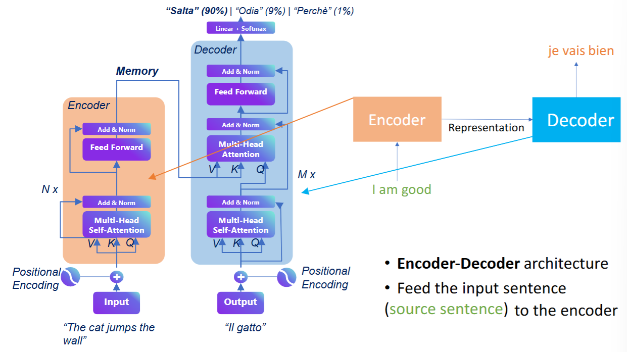
Encoder 与 Decoder：

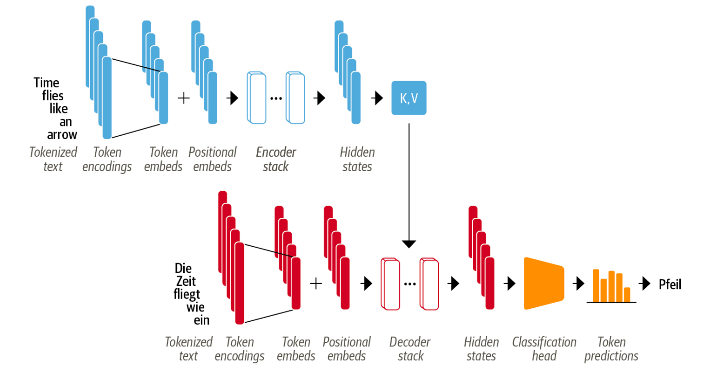
encoder only: seq of text -> rich representation (bidirectional attention)
- task
  - text classification
  - NER
- models
  - BERT
  - RoBERTa
  - DistilBERT
- 完形填空（bidirectional）
  - representation of a given token depends both on
    - left (before the token)
    - right (after the token)
decoder only (causal or autoregressive attention)
- GPT
- 词语接龙
- representation of a given token depends only on the left context
encoder-decoder
- tasks
  - machine translation
  - summarization
- models
  - T5
  - BART

我们上面是列举了 Transformer 的三种变体：

1.1 Encoder-only#

1
输入文本 → 丰富的语义表示（双向注意力）

注意力方式：双向，每个词在计算表示时，可以看到它 左边和右边 的所有词；
典型任务：
- 文本分类
- NER（命名实体识别）
代表模型：BERT, RoBERTa，DistilBERT

形象来说，encoder-only 的任务像是“完形填空”。比如句子 “I ____ you”，BERT 要预测 ____ 是什么词，它就会同时看：

左边的词 I
右边的词 you

两边都看，所以叫双向，这样能更好地理解整个句子的语义。

1.2 Decoder-only#

1
注意力只依赖于左边的上下文（因果注意力）

注意力方式：因果 / 自回归（causal / autoregressive），每个词在生成时，只能看到它左边（已经生成的）词，看不到右边的（因为右边还没生成）。
代表模型：GPT 系列

形象来说，decoder-only 的任务像是“词语接龙”，比如 GPT 要生成下一个词：“今天天气真__”.

它只能根据前面已经写出的 今天天气真 来预测下一个词是 好，热 还是 不错。它看不到后面还没写出来的词，所以叫单向的因果注意力。

1.3 Encoder-Decoder#

这就是我们上一段看到的经典 seq2seq 结构，最完整的 Transformer.

工作方式：Encoder 先用双向注意力把输入理解好 → Decoder 再用单向注意力逐步生成输出。
典型任务：
- 机器翻译（英→中）
- 文本摘要（长文→短摘要）
代表模型：T5、BART

2. encoder (encoder layer stack)#

encoder layer: encoding the contextual information (CNN)
- input: seq of embeddings
  - multi-head self attention
  - FFN (fully-connected)
- output:
  - same shape as input
- contextual information (contextualized embeddings)
  - apple: company-like or fruit-like ?
    - keynote
    - phone
  - files
    - time flies like an arrowL soars
    - fruit likes a banana: insect
skip connection (residual connection) & layer normalization
- 高效训练深度神经网络的技巧。

Transformer 的 Encoder 并不是一个单独的大模块，而是由 N 层相同的 Encoder Layer 堆叠而成，比如我们之前介绍的 BERT-base 模型就有 12 个 Transformer 层。

每一层 Encoder Layer 的结构如下：

1
输入：一串 embedding 向量
2
    │
3
    ├─ ❶ Multi-Head Self-Attention（多头自注意力）
4
    │
5
    ├─ ❷ Skip Connection + Layer Normalization（残差连接 + 层归一化）
6
    │
7
    ├─ ❸ Feed-Forward Network（前馈神经网络 / FC 全连接层）
8
    │
9
    ├─ ❹ Skip Connection + Layer Normalization
10
    │
11
输出：与输入形状相同的向量（但包含了上下文信息）

它的特点是 输出形状与输入形状相同，所以可以一层接一层地堆叠下去。

关于上下文信息（contextualized embeddings）部分，我们上面举了两个例子：

1
apple 是"苹果公司"还是"水果"？看周围词：
2

3
- keynote, phone → 像公司
4
- 如果是 eat, red → 像水果

可以看到，同一个词 apple，在不同句子中含义不同。Self-Attention 的作用就是：让 apple 去看它周围的词，根据上下文来确定它的语义。所以输出的向量不再是固定的词向量，而是融入了上下文信息的动态向量，这就是 contextualized embeddings（上下文感知的词向量）。

在另一个例子中，我们引用了一句经典的 NLP 例子：

1
Time flies like an arrow; fruit flies like a banana.

“时光如箭”，“果蝇喜欢香蕉”。同样，同一个词 flies，在两句中含义完全不同。Self-Attention 通过看周围的词（Time vs Fruit），就能正确区分。

残差连接（Skip Connection）与层归一化（Layer Normalization）是两个高效训练深度神经网络的技巧，它们的具体作用是：

技巧	作用	通俗理解
残差连接	让梯度能直接”跳过”某一层反向传播	像给网络加了”快捷通道”，防止层数太深导致梯度消失/爆炸
层归一化	把每层的输出拉回到标准范围内	让训练更稳定，收敛更快

2.1 multi-head self-attention layer#

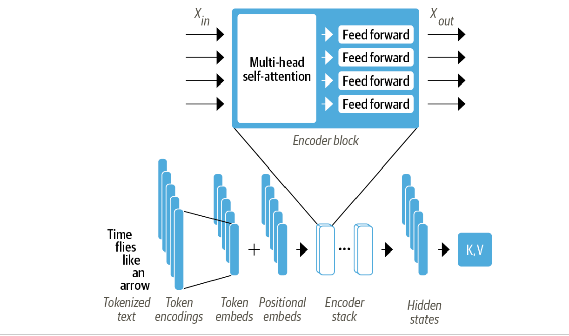
2.1.1 self-attention#

each token
- 不是 fixed embeddings
- 而是 weighted average of each embedding of the whole input sequence
a seq of token embedding: $x_1, x_2, ..., x_n$ , 经过 self-attention 得到 a seq of updated embeddings: $x_1^{'}, x_2^{'}, ..., x_n^{'}$ .

x_i^{'} = \sum_{j=1}^n w_{ji}x_j

$w_{ji}$ $w_{j i}$
- attention weights
- $\sum_j w_{ji}=1$
- $w\in \mathcal{R}^{n\times n}$

在 Self-Attention 之前，词向量（如 Word2Vec、GloVe）是固定的——“apple”永远只有一个向量，无论它在什么句子中。

但在 Self-Attention 中，每个词的新表示 = 句子中所有词的加权平均。

也就是说，apple 的新向量会融合句子里其他词的信息。如果句子里有 keynote、phone，那 apple 会偏向”公司”的含义；如果有 eat、red，则偏向”水果”的含义。

关于上面的数学公式，它的意思是：

我们输入词向量序列 $x_1, x_2, ..., x_n$
经过 self-attention 后得到 $x_1^{'}, x_2^{'}, ..., x_n^{'}$

我们可以用一个句子来理解。假设句子是 “I love you”，有 3 个词：

$x_1,x_2,x_3$ ：输入的词向量，即 “I”, “love” 和 “you” 的原始向量；
$x_1^{'}, x_2^{'}, x_3^{'}$ ：更新后的词向量，即 融入了上下文 后的新向量；
$w_{ji}$ ：这是 attention weight，表示词 $j$ 对词 $i$ 的“重要性”。

我们以 $x_2^{'}$ （“love” 的新向量）为例：

x_2^{'} = w_{12}x_1 + w_{22}x_2 + w_{32}x_3

展开来就是：

x_{love}^{'} = w_{I→love}·x_I + w_{love→love}·x_{love} + w_{you→love}·x_{you}

也就是说：“love” 的新向量 = “I”的信息 × 权重 + “love”自身的信息 × 权重 + “you”的信息 × 权重

如果权重显示 “I” 和 “you” 与 “love” 关系很紧密（比如 $w_{12}=0.4, w_{32}=0.4$ ），那么 $x_{love}^{'}$ 就会更多地融入”I”和”you”的信息。

关于权重 $w_{ji}$ 的性质：

性质	含义
$w_{ji}$	词 $j$ 对词 $i$ 的注意力权重
$\sum_j w_{ji}=1$	所有词对词 $i$ 的权重之和为 1（像概率一样）
$w \in \mathcal{R}^{n \times n}$	全部权重构成一个 $n \times n$ 的矩阵

这个 $n \times n$ 的权重矩阵可以直观理解为：

1
          I    love   you
2
    I  [ w₁₁   w₁₂   w₁₃ ]    ← "I" 看各个词
3
  love  [ w₂₁   w₂₂   w₂₃ ]    ← "love" 看各个词
4
   you  [ w₃₁   w₃₂   w₃₃ ]    ← "you" 看各个词

每一列是”这个词关注其他词的程度”，且每列之和 = 1。

比如第 2 列 $[w_{12}, w_{22}, w_{32}]^T$ 就是”love”对其他 3 个词的注意力分布。

2.1.2 scaled dor-product attention#

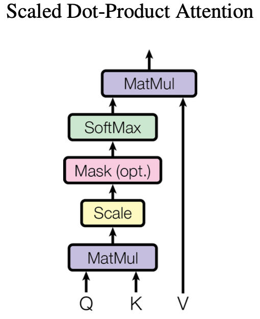
Attention(Q,K,V)=softmax(\frac{QK^T}{\sqrt{d_k}})V

Project each token embedding into 3 vectors called Query, Key and Value.
Compute attention scores.
- dot-product (Query, Key) -> attention scores;
- a seq with $n$ input tokens there is a corresponding $\mathcal{R}^{n\times n}$ matrix of attention scores.
Compute attention weights from attention scores: $w_{ji}$ $w_{j i}$
- Dot products 的结果可能是任意大的数，会让整个训练过程非常不稳定；
- 将 attention scores 乘以一个 scaling factor
- 然后 softmax 归一化： $\sum_j w_{ji}=1$
update the final embedding of the token (Value)
- $x_i^{'}=\sum_{j=1}^n w_{ji}v_j$

如同我们在 09 节中介绍过的那样，Self-attention 中权重 $w_{ji}$ 的计算分为清晰的 3 步：

1
每个 token 的向量
2
    ↓
3
第一步：投影出 3 个向量 → Query / Key / Value
4
    ↓
5
第二步：Query 与 Key 做点积 → attention scores → scaling → softmax → attention weights
6
    ↓
7
第三步：用 attention weights 对 Value 加权求和 → 得到最终输出

下面逐一展开。

① Query、Key、Value（查询、键、值）#

Project each token embedding into 3 vectors called Query, Key and Value.

对于每个输入的词向量 $x_i$ ，我们通过三个不同的权重矩阵 $W^Q, W^K, W^V$ ，把它分别投影成三个向量：

q_i = W^Q x_i \quad \text{(Query)}

k_i = W^K x_i \quad \text{(Key)}

v_i = W^V x_i \quad \text{(Value)}

为什么要分成三个角色？ 用一个生活类比：

角色	类比	作用
Query（查询）	🧐 你（读者）在图书馆搜索一本书	当前词”想找什么信息”
Key（键）	📚 每本书的书名标签	其他词”有什么信息可以给”
Value（值）	📖 书的内容本身	其他词”实际提供的信息内容”

以句子 “I love you” 为例，当处理 love 这个词时：

love 的 Query 负责问：“谁跟我有关系？”
I 和 you 的 Key 负责回答：“我在这里，我叫’I’ / ‘you’”
Query 和 Key 的匹配程度决定了 attention 权重
最后用权重去加权 Value（实际信息内容），得到 love 的新向量

② 计算 Attention Scores → Attention Weights#

dot-product (Query, Key) → attention scores

句子有 $n$ 个词，我们会得到一个 $n \times n$ 的 attention scores 矩阵。

对于词 $j$ 对词 $i$ 的得分（词 $i$ 查询词 $j$ ）：

\text{score}_{ji} = q_j \cdot k_i

点积越大 → Query 和 Key 越匹配 → 词 $j$ 越应该关注词 $i$ 。

为什么要除以 scaling factor？#

Dot products 的结果可能是任意大的数，会让整个训练过程非常不稳定

如果向量维度 $d_k$ 很大，点积的结果会非常大（因为很多数相加）。极端数值经过 softmax 后，会让大的更大、小的几乎消失，梯度变得非常小，模型学不动。

所以除以 $\sqrt{d_k}$ （scaling factor），把数值拉回合理范围：

\text{scaled score}_{ji} = \frac{q_j \cdot k_i}{\sqrt{d_k}}

然后 softmax 归一化#

w_{ji} = \frac{\exp(\text{scaled score}_{ji})}{\sum_{t=1}^n \exp(\text{scaled score}_{jt})}

经过 softmax 后， $\sum_j w_{ji} = 1$ ，变成一个概率分布——这就是我们之前公式里的 attention weights。

③ 用权重加权 Value，更新词向量#

$x_i^{'} = \sum_{j=1}^n w_{ji} v_j$

最后一步，用刚刚算出的权重 $w_{ji}$ 对 Value 向量 做加权求和：

x_{love}^{'} = w_{I→love}·v_I + w_{love→love}·v_{love} + w_{you→love}·v_{you}

注意这里用的是 $v_j$ （Value） 而不是原来的 $x_j$ 。这是因为 Value 是经过投影的”信息内容”，比原始向量更适合参与加权。

完整流程一图流#

1
输入:   x₁ (I)    x₂ (love)    x₃ (you)
2
          │          │           │
3
     ─────┴──────────┴───────────┴────
4
     │    W^Q        W^K         W^V  │   ← 三个投影矩阵
5
     ─────┬──────────┬───────────┬────
6
          │          │           │
7
          v          v           v
8
         qᵢ         kᵢ          vᵢ
9

10
Step 1:   q₂ · k₁   q₂ · k₂   q₂ · k₃     ← Query 与所有 Key 做点积
11
               ↓
12
Step 2:   [s₁, s₂, s₃] ÷ √dₖ → softmax → [w₁, w₂, w₃]   ← scaling + softmax
13
               ↓
14
Step 3:   x₂' = w₁·v₁ + w₂·v₂ + w₃·v₃     ← 加权求和 Value

2.1.3 visualization analysis#

1
from transformers import AutoTokenizer

1
from bertviz.transformers_neuron_view import BertModel
2
from bertviz.neuron_view import show

1
model_ckpt = 'bert-base-uncased'
2
tokenizer = AutoTokenizer.from_pretrained(model_ckpt)
3

4
model = BertModel.from_pretrained(model_ckpt)

1
model

输出为：

1
BertModel(
2
  (embeddings): BertEmbeddings(
3
    (word_embeddings): Embedding(30522, 768, padding_idx=0)
4
    (position_embeddings): Embedding(512, 768)
5
    (token_type_embeddings): Embedding(2, 768)
6
    (LayerNorm): BertLayerNorm()
7
    (dropout): Dropout(p=0.1, inplace=False)
8
  )
9
  (encoder): BertEncoder(
10
    (layer): ModuleList(
11
      (0-11): 12 x BertLayer(
12
        (attention): BertAttention(
13
          (self): BertSelfAttention(
14
            (query): Linear(in_features=768, out_features=768, bias=True)
15
            (key): Linear(in_features=768, out_features=768, bias=True)
16
            (value): Linear(in_features=768, out_features=768, bias=True)
17
            (dropout): Dropout(p=0.1, inplace=False)
18
          )
19
          (output): BertSelfOutput(
20
            (dense): Linear(in_features=768, out_features=768, bias=True)
21
            (LayerNorm): BertLayerNorm()
22
            (dropout): Dropout(p=0.1, inplace=False)
23
          )
24
        )
25
        (intermediate): BertIntermediate(
26
          (dense): Linear(in_features=768, out_features=3072, bias=True)
27
        )
28
        (output): BertOutput(
29
          (dense): Linear(in_features=3072, out_features=768, bias=True)
30
          (LayerNorm): BertLayerNorm()
31
          (dropout): Dropout(p=0.1, inplace=False)
32
        )
33
      )
34
    )
35
  )
36
  (pooler): BertPooler(
37
    (dense): Linear(in_features=768, out_features=768, bias=True)
38
    (activation): Tanh()
39
  )
40
)

这是我们之前介绍过许多次的经典 BERT 模型架构。

1
sample_text = 'time flies like an arrow'
2

3
show(
4
    model,
5
    model_type='bert',
6
    tokenizer=tokenizer,
7
    sentence_a=sample_text,
8
    display_mode='light',
9
    layer=0,
10
    head=8
11
    )

这里输出的是一个可交互的页面，让我们可以直观地看到每个词关注了哪些词。我们来大致解释一下 show() 里面的参数：

model ：加载的 BERT 模型，用来前向传播计算 attention 权重；
model_type='bert' ：告诉 BertViz 你用的是哪种模型架构。因为 BertViz 支持多种模型（bert、gpt2、xlnet 等），每种模型的内部结构略有不同，需要指定类型才能正确解析 attention 矩阵；
tokenizer ：分词器，用于把输入的句子转成 token IDs，同时知道每个 token 对应的文本是什么，方便在可视化中显示标签；
sentence_a ：要可视化的句子。sentence_a 这个命名来自 BERT 的预训练任务——它本来可以接收两个句子（比如 NSP 任务），这里只需要一个句子所以只用 sentence_a；
display_mode ：可视化界面的主题风格。'light' 是浅色背景，还有 'dark' 深色模式可选。
layer=0 ：选择哪一层的 attention 来可视化。BERT-base 有 12 层（0~11），layer=0 就是第 1 层（最靠近输入的那一层）。不同层关注的模式不同：
- 浅层（layer 0~3）：更多关注语法关系、相邻词
- 中层（layer 4~7）：开始捕捉一定的语义
- 深层（layer 8~11）：关注高层次的语义关联
head ：选择第几个注意力头来可视化。Multi-Head Attention 有多个头（BERT-base 有 12 个头，编号 0~11），每个头关注不同的模式。比方说：

1
head 0 → 关注下一个词
2
head 5 → 关注句法依赖关系（如动词→名词）
3
head 8 → 关注句法关系（可能看到 "time" 关注 "flies" 的修饰关系）

不过实际上，选择 layer 和 head 只影响一开始展示的层和头。你可以在可交互页面的上端选择自由查看每一层和每个头。

2.1.4 computation of self-attention#

1
model_inputs = tokenizer(sample_text, return_tensors='pt', add_special_tokens=False)
2
model_inputs

输出为：

1
{'input_ids': tensor([[ 2051, 10029,  2066,  2019,  8612]]), 'token_type_ids': tensor([[0, 0, 0, 0, 0]]), 'attention_mask': tensor([[1, 1, 1, 1, 1]])}

注意这里我们没有加入 [CLS] 和 [SEP] 特殊 token.

1
from torch import nn
2
from transformers import AutoConfig

1
config = AutoConfig.from_pretrained(model_ckpt)
2
config

输出为：

1
BertConfig {
2
  "add_cross_attention": false,
3
  "architectures": [
4
    "BertForMaskedLM"
5
  ],
6
  "attention_probs_dropout_prob": 0.1,
7
  "bos_token_id": null,
8
  "classifier_dropout": null,
9
  "eos_token_id": null,
10
  "gradient_checkpointing": false,
11
  "hidden_act": "gelu",
12
  "hidden_dropout_prob": 0.1,
13
  "hidden_size": 768,
14
  "initializer_range": 0.02,
15
  "intermediate_size": 3072,
16
  "is_decoder": false,
17
  "layer_norm_eps": 1e-12,
18
  "max_position_embeddings": 512,
19
  "model_type": "bert",
20
  "num_attention_heads": 12,
21
  "num_hidden_layers": 12,
22
  "pad_token_id": 0,
23
  "position_embedding_type": "absolute",
24
  "tie_word_embeddings": true,
25
  "transformers_version": "5.9.0",
26
  "type_vocab_size": 2,
27
  "use_cache": true,
28
  "vocab_size": 30522
29
}

以上就是 BERT 模型中的超参数，它们定义了 BERT 的骨架。需要注意的是，这里并不是 BERT 模型全部的超参数，训练的超参数需要在训练脚本（例如 HuggingFace 的 Trainer 中设置），比如学习率、优化器、batch_size 等等。

下面我们简单介绍一下每个参数的含义：

核心结构参数（最重要的）：

参数	值	含义
`hidden_size`	768	每个 token 的隐藏层向量维度。即输入/输出的 embedding 长度
`num_hidden_layers`	12	Encoder Layer 堆叠的层数
`num_attention_heads`	12	Multi-Head Attention 的头数。每头的维度 = 768/12 = 64
`intermediate_size`	3072	FFN 中间层的维度（先放大到 3072，再缩小回 768 = 4× 关系）
`vocab_size`	30522	词汇表大小，即 `word_embeddings` 矩阵的行数
`max_position_embeddings`	512	最大输入序列长度

激活函数 & Dropout：

参数	值	含义
`hidden_act`	gelu	FFN 中的激活函数，不是 ReLU，是 GELU（高斯误差线性单元）
`hidden_dropout_prob`	0.1	隐藏层的 Dropout 概率
`attention_probs_dropout_prob`	0.1	Attention 权重上的 Dropout 概率
`classifier_dropout`	null	分类头专用 Dropout（此处未单独设置）

特殊 Token & 位置编码：

参数	值	含义
`pad_token_id`	0	padding token 的 ID
`bos_token_id`	null	序列开始 token（BERT 不用，用 [CLS]）
`eos_token_id`	null	序列结束 token（BERT 不用）
`position_embedding_type`	absolute	位置编码方式：绝对位置编码
`type_vocab_size`	2	token type 数量（区分两个句子的 [0, 1]）

其他配置：

参数	值	含义
`is_decoder`	false	不是 decoder，是 encoder-only
`layer_norm_eps`	1e-12	Layer Norm 的分母微小值，防止除零
`initializer_range`	0.02	参数初始化的范围（截断正态分布）
`gradient_checkpointing`	false	是否用梯度检查点节省显存（慢但省显存）
`tie_word_embeddings`	true	是否绑定输入/输出 embedding 权重（BERT 用于 MLM）
`add_cross_attention`	false	是否添加 cross-attention（encoder-decoder 需要）
`use_cache`	true	是否缓存 KV（decoder 生成时加速用）

1
# config.vocab_size: 30522
2
# config.hidden_size: 768=64*12
3
token_embedding = nn.Embedding(config.vocab_size, config.hidden_size)
4
token_embedding # Embedding(30522, 768)

1
# forward of embedding module
2
input_embeddings = token_embedding(model_inputs['input_ids'])
3

4
# batch_size, seq_len, hidden_size
5
input_embeddings.shape # torch.Size([1, 5, 768])

1
# 先不考虑 position encoding
2
# query: [1, 5, 768], key: [1, 5, 768], value: [1, 5, 768]
3
# W_q, W_k, W_v: nn.linear, 作用在 token_embedding 上，依然通过 learing 最终决定
4
query = key = value = input_embeddings
5
dim_k = key.size(-1) # 768
6
print(dim_k)
7

8
# /np.sqrt(dim_k) 是为了缩放，防止 dot product 过大导致 softmax 后梯度消失
9
attention_scores = torch.matmul(query, key.transpose(1, 2)) / np.sqrt(dim_k)
10
attention_scores.shape # torch.Size([1, 5, 5])
11
attention_scores

输出为：

1
tensor([[[27.1932,  1.1826, -0.4651,  0.3558,  0.2249],
2
         [ 1.1826, 29.3970, -0.2585,  2.2841,  1.1054],
3
         [-0.4651, -0.2585, 26.4902, -0.1578, -0.9823],
4
         [ 0.3558,  2.2841, -0.1578, 28.4970,  1.3951],
5
         [ 0.2249,  1.1054, -0.9823,  1.3951, 26.8615]]],
6
       grad_fn=<DivBackward0>)

这里我们得到的就是注意力分数矩阵，也就是公式中 $\frac{QK^T}{\sqrt{d_k}}$ 这一步的结果。

可以看出，对角线的值远远大于非对角线。这是因为每个词语自己最相似，所以点积最大。

需要注意的是，我们没有用可学习的 $W^Q, W^K$ 投影，而是直接 query = key = value = input_embeddings，相当于 $X\cdot X^T/\sqrt{d_k}$ ，即每个 token 与其他所有 token 的点积。所以，这些分数只反映了 原始 token embedding 的余弦相似度，还不是真正经过学习的 attention.

如果采用 $W^Q, W^K$ 投影，它们会这些分数”调教”成更有语义意义的注意力分布——比如让 flies 更关注 time（语法修饰关系），而不是全靠自身。

1
# from scores -> weights, softmax
2
import torch.nn.functional as F
3

4
attention_weights = F.softmax(attention_scores, dim=-1)
5
attention_weights.shape # torch.Size([1, 5, 5])
6
attention_weights

输出为：

1
tensor([[[1.0000e+00, 5.0553e-12, 9.7307e-13, 2.2112e-12, 1.9401e-12],
2
         [5.5803e-13, 1.0000e+00, 1.3206e-13, 1.6789e-12, 5.1658e-13],
3
         [1.9655e-12, 2.4165e-12, 1.0000e+00, 2.6727e-12, 1.1718e-12],
4
         [6.0036e-13, 4.1294e-12, 3.5925e-13, 1.0000e+00, 1.6974e-12],
5
         [2.7034e-12, 6.5209e-12, 8.0838e-13, 8.7118e-12, 1.0000e+00]]],
6
       grad_fn=<SoftmaxBackward0>)

这里就是上一步的 attention_scores 经过 softmax 归一化后的结果，也就是我们之前提到过的 $w_{ji}$ .

不过这里我们会发现：

1
        time    flies   like    an      arrow
2
time    1.00    ~0      ~0      ~0      ~0
3
flies   ~0      1.00    ~0      ~0      ~0
4
like    ~0      ~0      1.00    ~0      ~0
5
an      ~0      ~0      ~0      1.00    ~0
6
arrow   ~0      ~0      ~0      ~0      1.00

几乎每个词都 100% 关注自己，而不看其他任何词。

这是我们前面简化的结果，在这种简化下，每个 token 和自己一模一样，点积当然远远大于与其他 token 的点积。这样的 attention 是完全失效的——每个词都是”孤岛”，没有吸收任何上下文信息。

不过，这里我们只是演示计算的过程，只需要知道真实的 BERT 并不是这样的即可。

1
attention_weights.sum(dim=-1) # 每行加起来等于 1

输出为：

1
tensor([[1., 1., 1., 1., 1.]], grad_fn=<SumBackward1>)

可以看到，经过 softmax 归一化后，每行加起来都等于 1，也就对应前面我们提到过的 $\sum_j w_{ji}=1$ .

1
# 5*5, 5*768 -> 5*768
2
attention_output = torch.bmm(attention_weights, value)
3
attention_output.shape # torch.Size([1, 5, 768])
4
attention_output

输出为：

1
tensor([[[-0.3932,  0.1078, -1.3741,  ..., -0.8332,  1.7649, -0.8743],
2
         [-1.7124, -1.0425, -0.7992,  ...,  0.6528,  0.5512,  1.1871],
3
         [-1.1721, -1.1326,  0.3345,  ..., -0.1074,  0.3040, -0.2598],
4
         [-0.4535, -0.7321, -1.8562,  ..., -0.1357,  1.2970,  0.2048],
5
         [-0.6879, -1.6019,  0.6278,  ...,  0.2712,  0.0040, -0.2760]]],
6
       grad_fn=<BmmBackward0>)

这里我们就来到了公式中的最后一步，用 attention_weights 对 Value 进行加权求和，形状为 (1, 5, 768)：

1 个 batch
5 个 token
每个 768 维

同样，由于我们简化的结果：

1
x₁' = 1.0 · v₁ + 0 · v₂ + 0 · v₃ + 0 · v₄ + 0 · v₅ = v₁
2
x₂' = 0 · v₁ + 1.0 · v₂ + 0 · v₃ + 0 · v₄ + 0 · v₅ = v₂
3
...

输出的每一行，其实就等于对应 token 自己的 Value 向量，几乎没有从其他词吸收任何信息。

我们用一个完整的函数覆盖上述步骤：

1
# batch_size, seq_len, hidden_size
2
def scaled_dot_product_attention(query, key, value):
3
    dim_k = key.size(-1)
4
    attention_scores = torch.matmul(query, key.transpose(1, 2)) / np.sqrt(dim_k)
5
    attention_weights = F.softmax(attention_scores, dim=-1)
6
    attention_output = torch.bmm(attention_weights, value)
7
    return attention_output

1
scaled_dot_product_attention(query, key, value)

输出为：

1
tensor([[[-0.3932,  0.1078, -1.3741,  ..., -0.8332,  1.7649, -0.8743],
2
         [-1.7124, -1.0425, -0.7992,  ...,  0.6528,  0.5512,  1.1871],
3
         [-1.1721, -1.1326,  0.3345,  ..., -0.1074,  0.3040, -0.2598],
4
         [-0.4535, -0.7321, -1.8562,  ..., -0.1357,  1.2970,  0.2048],
5
         [-0.6879, -1.6019,  0.6278,  ...,  0.2712,  0.0040, -0.2760]]],
6
       grad_fn=<BmmBackward0>)

最后，补充介绍一下 .matmul() 与 .bmm() 函数：

torch.matmul() ：通用矩阵乘法，支持多种维度的输入，会根据输入自动选择计算方式：

输入维度	行为	例子
两个 2D `(m, n) × (n, p)`	标准矩阵乘法	→ `(m, p)`
3D + 2D `(b, m, n) × (n, p)`	批次广播	→ `(b, m, p)`
两个 3D `(b, m, n) × (b, n, p)`	批次矩阵乘法	→ `(b, m, p)`
1D 向量	点积

之前我们用的就是 3D 版本：

1
# query: [1, 5, 768], key.transpose: [1, 768, 5]
2
torch.matmul(query, key.transpose(1, 2))  # → [1, 5, 5]

torch.bmm() ：专门用于 3D 张量的批次矩阵乘法，要求输入必须恰好是 3D：

1
torch.bmm(attention_weights, value)
2
# weights: [1, 5, 5],  value: [1, 5, 768]
3
# → output: [1, 5, 768]

二者关键区别：

	`matmul()`	`bmm()`
输入维度	灵活（1D~3D+）	必须两个都是 3D
广播	✅ 支持	❌ 不支持（batch 维必须相等）
使用场景	Q 与 K^T 相乘（维数可能不同）	weights 与 V 相乘（都是明确 3D）

简单来说：matmul 通用灵活，bmm 专一高效。二者在 3D 输入且 batch 一致时的行为等价，但 bmm 更严格——如果你确定两个输入都是 (batch, n, m) 形状，用 bmm 可以提前捕捉维度错误。

音乐

音乐

1. summary#

1.1 Encoder-only#

1.2 Decoder-only#

1.3 Encoder-Decoder#

2. encoder (encoder layer stack)#

2.1 multi-head self-attention layer#

2.1.1 self-attention#

2.1.2 scaled dor-product attention#

① Query、Key、Value（查询、键、值）#

② 计算 Attention Scores → Attention Weights#

为什么要除以 scaling factor？#

然后 softmax 归一化#

③ 用权重加权 Value，更新词向量#

完整流程一图流#

2.1.3 visualization analysis#

2.1.4 computation of self-attention#

文章分享

评论区

音乐

文章目录

音乐

音乐

02_transformer_architecture_self_attention

1. summary#

1.1 Encoder-only#

1.2 Decoder-only#

1.3 Encoder-Decoder#

2. encoder (encoder layer stack)#

2.1 multi-head self-attention layer#

2.1.1 self-attention#

2.1.2 scaled dor-product attention#

① Query、Key、Value（查询、键、值）#

② 计算 Attention Scores → Attention Weights#

为什么要除以 scaling factor？#

然后 softmax 归一化#

③ 用权重加权 Value，更新词向量#

完整流程一图流#

2.1.3 visualization analysis#

2.1.4 computation of self-attention#

文章分享

评论区

音乐

文章目录